Scilab 5.5.0
- Aide de Scilab
- CACSD (Computer Aided Control Systems Design)
- Représentations formelles et conversions
- Plot and display
- noisegen
- pol2des
- syslin
- abinv
- arhnk
- arl2
- arma
- arma2p
- arma2ss
- armac
- armax
- armax1
- arsimul
- augment
- balreal
- bilin
- bstap
- cainv
- calfrq
- canon
- ccontrg
- cls2dls
- colinout
- colregul
- cont_mat
- contr
- contrss
- copfac
- csim
- ctr_gram
- damp
- dcf
- ddp
- dhinf
- dhnorm
- dscr
- dsimul
- dt_ility
- dtsi
- equil
- equil1
- feedback
- findABCD
- findAC
- findBD
- findBDK
- findR
- findx0BD
- flts
- fourplan
- freq
- freson
- fspec
- fspecg
- fstabst
- g_margin
- gamitg
- gcare
- gfare
- gfrancis
- gtild
- h2norm
- h_cl
- h_inf
- h_inf_st
- h_norm
- hankelsv
- hinf
- imrep2ss
- inistate
- invsyslin
- kpure
- krac2
- lcf
- leqr
- lft
- lin
- linf
- linfn
- linmeq
- lqe
- lqg
- lqg2stan
- lqg_ltr
- lqr
- ltitr
- macglov
- minreal
- minss
- mucomp
- narsimul
- nehari
- nyquistfrequencybounds
- obs_gram
- obscont
- observer
- obsv_mat
- obsvss
- p_margin
- parrot
- pfss
- phasemag
- plzr
- ppol
- prbs_a
- projsl
- repfreq
- ric_desc
- ricc
- riccati
- routh_t
- rowinout
- rowregul
- rtitr
- sensi
- sident
- sorder
- specfact
- ssprint
- st_ility
- stabil
- sysfact
- syssize
- time_id
- trzeros
- ui_observer
- unobs
- zeropen
Please note that the recommended version of Scilab is 2026.1.0. This page might be outdated.
See the recommended documentation of this function
kpure
continuous SISO system limit feedback gain
Calling Sequence
K=kpure(sys [,tol])
[K,R]=kpure(sys [,tol])
Arguments
- sys
SISO linear system (syslin)
- tol
a positive scalar. tolerance used to determine if a root is imaginary or not. The default value is
1e-6- K
Real vector, the vector of gains for which at least one closed loop pole is imaginary.
- R
Complex vector, the imaginary closed loop poles associated with the values of
K.
Description
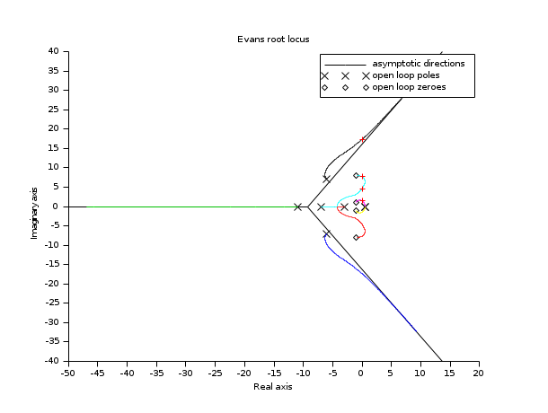
K=kpure(sys) computes the gains K such that the system
sys feedback by K(i) (sys/.K(i)) has poles on imaginary axis.
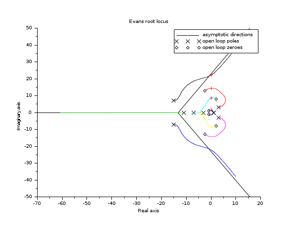
Examples
num=real(poly([-1+%i, -1-%i, -1+8*%i  -1-8*%i],'s'));
den=real(poly([0.5 0.5  -6+7*%i  -6-7*%i  -3 -7 -11],'s'));
h=num/den;

[K,Y]=kpure(h)
clf();evans(h)
plot(real(Y),imag(Y),'+r')
num=real(poly([-1+%i*1, -1-%i*1, 2+%i*8  2-%i*8 -2.5+%i*13 -2.5-%i*13],'s'));
den=real(poly([1 1 3+%i*3 3-%i*3 -15+%i*7  -15-%i*7  -3 -7 -11],'s'));
h=num/den;

[K,Y]=kpure(h)
clf();evans(h,100000)
plot(real(Y),imag(Y),'+r')
| Report an issue | ||
| << invsyslin | CACSD (Computer Aided Control Systems Design) | krac2 >> |