plot
2Dプロット
呼び出しの手順
plot // demo
plot(y)
plot(x, y)
plot(x, func)
plot(x, list(func, params))
plot(x, polynomial)
plot(x, rational)
plot(.., LineSpec)
plot(.., LineSpec, GlobalProperty)
plot(x1, y1, LineSpec1, x2,y2,LineSpec2,...xN, yN, LineSpecN, GlobalProperty1,.. GlobalPropertyM)
plot(x1,func1,LineSpec1, x2,y2,LineSpec2,...xN,funcN,LineSpecN, GlobalProperty1, ..GlobalPropertyM)
plot(logflag,...)
plot(axes_handle,...)
引数
- x
実数行列またはベクトル. 省略した場合,
1:nであると 仮定されます. ただし,nはyパラメータで 指定された曲線の点の数です.- y
- 実数行列またはベクトル.
- func
handle of a function, as in
plot(x, sin). If the function to plot needs some parameters as input arguments, the function and its parameters can be specified through a list, as inplot(x, list(delip, -0.4))- polynomial
- Single polynomial or array of polynomials.
- rational
- Single rational or array of rationals.
- y1, y2, y3,..
Can be any of the possible input types described above:
- vectors or matrices of real numbers or of integers
- handle of a function (possibly in a list with its parameters).
- polynomials
- rationals
- LineSpec
このオプション引数は文字列で 線を描画する手法を指定するショートカットとして使用されます.
LineSpecは指定済みの各yまたは{x,y}毎に一つ指定できます.LineSpecはLineStyle,MarkerおよびColorと同時に処理されます (LineSpec参照). これらの指定子はプロットされた線において線の種類,マーカの種類および色を定義します.- GlobalProperty
このオプションの引数は, グローバルオブジェクトのプロパティを定義する 一連の命令
{PropertyName,PropertyValue}を表し, このプロットで作成された全ての曲線に適用されます. 利用可能なプロパティの全て参照するには GlobalPropertyを参照してください.- logflag
"ln" | "nl" | "ll" : 2-character word made of "l" standing for "Logarithmic" or/and "n" standing for "Normal". The first character applies to the X axis, the second to the Y axis. Hence, "ln" means that the X axis is logarithmic and the Y axis is normal. The default is "nn": both axes in normal scales.
logflagmust be used afteraxes_handle(if any) and before the first curve's dataxoryorfunc. It applies to all curves drawn by theplot(…)instruction.- axes_handle
このオプションの引数は,カレントの軸ではなく
axes_handleで 指定した軸の内部にプロットが表示されることを指定します (gca参照).
説明
plot は一連の二次元曲線をプロットします.
plot はMatlab構文との互換性を改善するために
修正されています.
グラフィックの互換性を改善するために, Matlabユーザは
(plot2dではなく)
plotを使用してください.
データエントリ仕様 :
本節では,記述を明確化するため,オプションの引数
LineSpecおよび GlobalProperty
については言及しません.
これはこれらの引数は,
("Xdata",
"Ydata" および "Zdata" プロパティを
除く,
GlobalProperty参照)
エントリデータと干渉しないためです.
これら全てのオプション引数を同時に指定することが可能です.
y がベクトルの場合, plot(y) はベクトル y
をベクトル 1:size(y,'*')に対してプロットします.
yが行列の場合, plot(y) はyの各列を
1:size(y,1)に対してプロットします.
x および y がベクトルの場合, plot(x,y) は
ベクトル y をベクトル xに対してプロットします.
ベクトルx および
y の要素数は同じである必要があります.
x がベクトルで y が行列の場合, plot(x,y)
は y の各列をベクトル xに対してプロットします.
この場合,y の列の数は
x のエントリの数と同じである必要があります.
x と y が行列の場合, plot(x,y) は
y の各列をxの同じ列に対してプロットします.
この場合,x とy の大きさは同じである必要があります.
最後に, x または y が行列の場合,
ベクトルは行列の各行または各列に対してプロットされます.
この選択は,行列の行また列の次元にベクトルの行または列の次元のどちらが
一致するかに応じて行われます.
(x または y のみが)正方行列の場合,
列が行よりも優先されます(以下の例参照).
 | 必要でかつ可能な場合,
plot は,
互換性がある次元を取得するため,
x および yを転置し,警告を出力します.
例えば,
x がyの列と同じ行数を有する場合.
y が正方の場合, 転置は行われません. |
y はマクロまたはプリミティブとして定義された関数と
することも可能です.この場合,
x データを(ベクトルまたは行列として)指定する必要があり,
対応するy(x)の計算が暗黙の内に行われます.
LineSpec とGlobalProperty 引数は
プロットをカスタマイズするために使用されます.
以下に利用可能な全オプションのリストを示します.
- LineSpec
このオプションは曲線の描画方法を簡便な方法で 指定する際に使用されます. このオプションは,LineStyle, Marker および Color指定子を含む文字列とする 必要があります.
これらのリファレンスは曖昧さがないように 文字列内で指定することが必要です(順番は重要ではありません). 例えば,ダイヤモンド型の記号を付けた赤い長い破線を指定する場合, 以下のように書くことができます:
'r--d','--dire'または'--reddiam'または他のあいまいでない命令, もしくは全体を指定する'diamondred--'(LineSpec参照)線の種類,色,マーカの色(および大きさ)も ポリラインエンティティプロパティにより(再)設定できることに 注意してください (polyline_properties参照).
- GlobalProperty
このオプションは,
LineSpecを使用する よりも多くのオプションを用いて曲線のプロット方法を指定できます.PropertyNameを定義する文字列と その値であるPropertyValue(PropertyNameの型に依存して文字列または整数または...) の組で指定する必要があります.GlobalPropertyにより複数のプロパティ, つまり, LineSpec により利用可能なあらゆるプロパティ, マーカの色(表示色および背景色), 視認性, クリッピング, 曲線の太さ, を設定可能です. (GlobalProperty参照)これらのプロパティは全て ポリラインエンティティプロパティ (polyline_properties参照) により(再)設定できることに注意してください.
注意
デフォルトでは, 連続したプロットは重ね描きされます.
前のプロットを消去するには,
clf()を使用してください. auto_clear モードを
デフォルトで有効にするには,次のようにデフォルトの軸を編集してください:
da=gda();
da.auto_clear = 'on'
表示を改善するためにplot関数が親の軸の
boxプロパティを修正することがあります.
これは,親の軸がplotのコールにより作成されたか,
コール前に空である場合に行われます.
軸の一つが原点を中心にしている場合, ボックスは無効となります.
その他の場合, ボックスが有効になります.
ボックスプロパティと軸の配置に関する詳細については, axes_propertiesを参照ください.
色を指定しない場合,曲線をプロットする際にデフォルトの色テーブルが 使用されます. 複数の線を描画する際,plotコマンドは自動的に このテーブルに基づき周期的に選択します. 以下に使用される色を示します:
R |
G |
B |
|---|---|---|
| 0. | 0. | 1. |
| 0. | 0.5 | 0. |
| 1. | 0. | 0. |
| 0. | 0.75 | 0.75 |
| 0.75 | 0. | 0.75 |
| 0.75 | 0.75 | 0. |
| 0.25 | 0.25 | 0.25 |
コマンド plot を入力することによりデモを見ることができます.
例
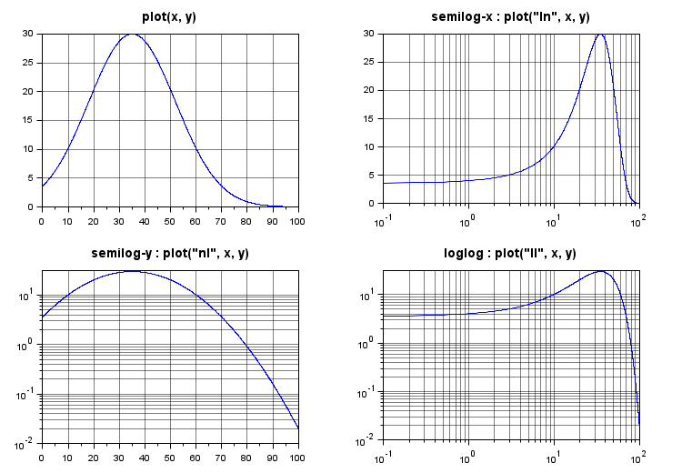
Choosing the normal or logarithmic plotting mode:
gda().grid = [1 1]*color("grey70");
title(gda(), "fontsize", 3, "color", "lightseagreen", "fontname", "helvetica bold");

x = linspace(1e-1,100,1000);
xm = 35;
dx = 17;
G = exp(-((x-xm)/dx).^2/2)*30;

scf(1); clf

subplot(2,2,1), plot(x, G),       title("plot(x, y)")
subplot(2,2,2), plot("ln", x, G), title("semilog-x : plot(""ln"", x, y)"); gca().sub_ticks(1) = 8;
subplot(2,2,3), plot("nl", x, G), title("semilog-y : plot(""nl"", x, y)"); gca().sub_ticks(2) = 8;
subplot(2,2,4), plot("ll", x, G), title("loglog : plot(""ll"", x, y)");    gca().sub_ticks = [8 8];

sda();
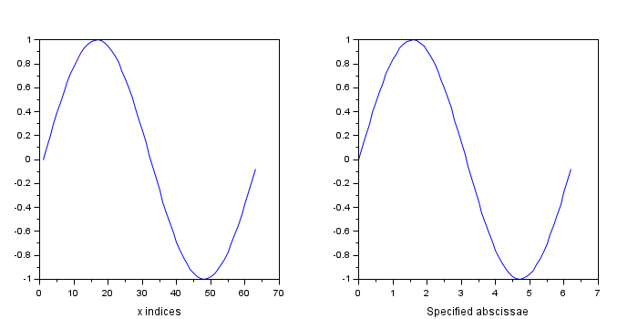
Simple plot of a single curve:
// Default abscissae = indices
subplot(1,2,1)
plot(sin(0:0.1:2*%pi))
xlabel("x indices")

// With explicit abscissae:
x = [0:0.1:2*%pi]';
subplot(1,2,2)
plot(x, sin(x))
xlabel("Specified abscissae")
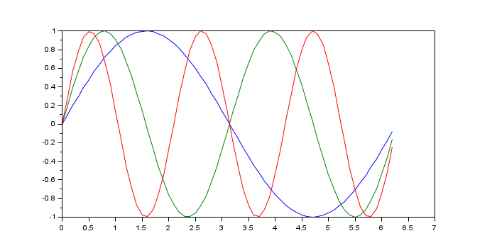
Multiple curves with shared abscissae: Y: 1 column = 1 curve:
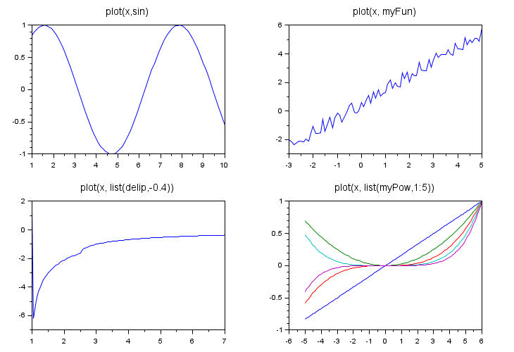
Specifying a macro or a builtin instead of explicit ordinates:
clf
subplot(2,2,1)         // sin() is a builtin
plot(1:0.1:10, sin)    // <=> plot(1:0.1:10, sin(1:0.1:10))
title("plot(x, sin)", "fontsize",3)

// with a macro:
deff('y = myFun(x)','y = x + rand(x)')
subplot(2,2,2)
plot(-3:0.1:5, myFun)
title("plot(x, myFun)", "fontsize",3)

// With functions with parameters:
subplot(2,2,3)
plot(1:0.05:7, list(delip, -0.4))  // <=> plot(1:0.05:7, delip(1:0.05:7,-0.4) )
title("plot(x, list(delip,-0.4))", "fontsize",3)

function Y=myPow(x, p)
    [X,P] = ndgrid(x,p);
    Y = X.^P;
    m = max(abs(Y),"r");
    for i = 1:size(Y,2)
        Y(:,i) = Y(:,i)/m(i);
    end
endfunction
x = -5:0.1:6;
subplot(2,2,4)
plot(x, list(myPow,1:5))
title("plot(x, list(myPow,1:5))", "fontsize",3)
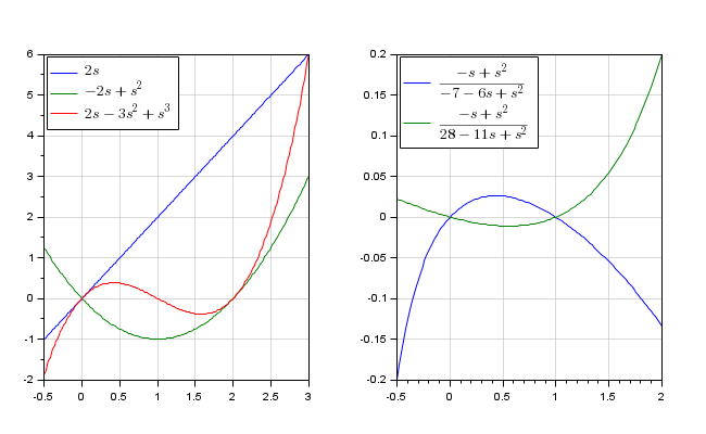
Plotting the graph of polynomials or rationals:
clf
s = %s;

// Polynomials
x = -0.5:0.02:3;
p = s*[2 ; (s-2) ; (s-1)*(s-2)]
subplot(1,2,1)
plot(x, p)
legend(prettyprint(p,"latex","",%t), 2);

// Rationals
x = -0.5:0.02:2;
r = (s-1)*s/(s-7)./[s+1, s-4]
subplot(1,2,2)
plot(x, r)
legend(prettyprint(r,"latex","",%t), 2);

gcf().children.grid = color("grey70")*[1 1]; // grids
gcf().children.children([1 3]).font_size=3;  // legends
--> p = s*[2 ; (s-2) ; (s-1)*(s-2)]
 p  =
  2s
  -2s +s²
  2s -3s² +s³

../..
--> r = (s-1)*s/(s-7)./[s+1, s-4]
 r  =
     -s +s²      -s +s²
   ----------  -----------
   -7 -6s +s²  28 -11s +s²
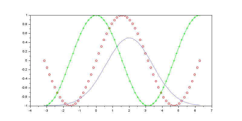
Setting curves simple styles when calling plot():
clf
t = -%pi:%pi/20:2*%pi;
// sin() : in Red, with O marks, without line
// cos() : in Green, with + marks, with a solid line
// gaussian: in Blue, without marks, with dotted line
gauss = 1.5*exp(-(t/2-1).^2)-1;

plot(t,sin,'ro', t,cos,'g+-', t,gauss,':b')
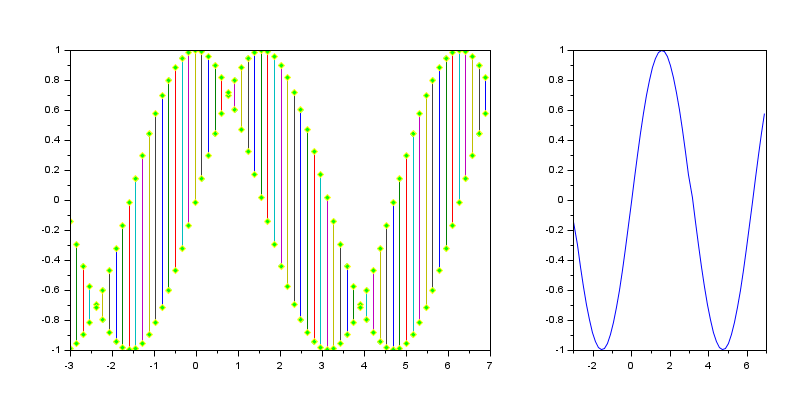
Vertical segments between two curves, with automatic colors, and using Global properties for markers styles. Targeting a defined axes.
clf
subplot(1,3,3)
ax3 = gca();         // We will draw here later
xsetech([0 0 0.7 1]) // Defines the first Axes area
t = -3:%pi/20:7;
// Tuning markers properties
plot([t ;t],[sin(t) ;cos(t)],'marker','d','markerFaceColor','green','markerEdgeColor','yel')

// Targeting a defined axes
plot(ax3, t, sin)
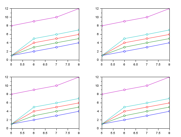
Case of a non-square Y matrix: When it is consistent and required, X or/and Y data are automatically transposed in order to become plottable.
clf()
x = [5 6 7 8]
y = [1   1   1   1   8
     2   3   4   5   9
     3   4   5   6  10
     4   5   6   7  12];

// Only one matching possibility case: how to make 4 identical plots in 4 manners...
// x is 1x4 (vector) and y is 4x5 (non square matrix)
subplot(221); plot(x', y , "o-");    // OK as is
subplot(222); plot(x , y , "o-");    // x is transposed
subplot(223); plot(x', y', "o-");    // y is transposed
subplot(224); plot(x , y', "o-");    // x and y are transposed
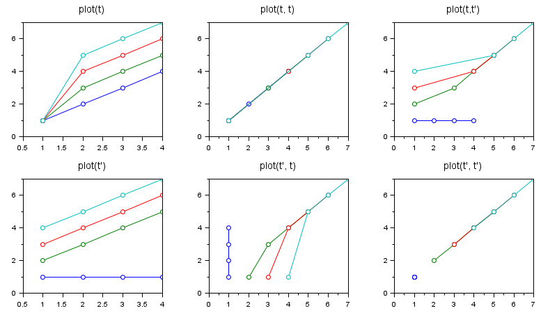
Case of a square Y matrix, and X implicit or square:
clf
t = [1   1   1   1
     2   3   4   5
     3   4   5   6
     4   5   6   7];

subplot(231), plot(t,"o-") , title("plot(t)",  "fontsize",3)
subplot(234), plot(t',"o-"), title("plot(t'')", "fontsize",3)

subplot(232), plot(t,t,"o-") , title("plot(t, t)",  "fontsize",3)
subplot(233), plot(t,t',"o-"), title("plot(t,t'')", "fontsize",3)

subplot(235), plot(t', t,"o-"),  title("plot(t'', t)",   "fontsize",3)
subplot(236), plot(t', t',"o-"), title("plot(t'', t'')", "fontsize",3)

for i=1:6, gcf().children(i).data_bounds([1 3]) = 0.5; end
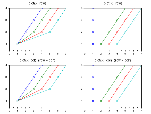
Special cases of a matrix X and a vector Y:
clf
X = [1   1   1   1
     2   3   4   5
     3   4   5   6
     4   5   6   7];
y = [1 2 3 4];

subplot(221), plot(X, y,  "o-"), title("plot(X, row)",  "fontsize",3)
        // equivalent to plot(t, [1 1 1 1; 2 2 2 2; 3 3 3 3; 4 4 4 4])
subplot(223), plot(X, y', "o-"), title("plot(X, col)  (row = col'')",  "fontsize",3)
subplot(222), plot(X',y,  "o-"), title("plot(X'', row)",  "fontsize",3)
subplot(224), plot(X',y', "o-"), title("plot(X'', col)  (row = col'')",  "fontsize",3)

for i = 1:4, gcf().children(i).data_bounds([1 3]) = 0.5; end
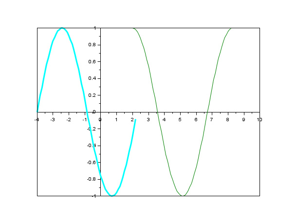
Post-tuning Axes and curves:
x=[0:0.1:2*%pi]';
plot(x-4,sin(x),x+2,cos(x))

// (0,0)を中心とする軸
a=gca(); // 軸エンティティのハンドル
a.x_location = "origin";
a.y_location = "origin";
isoview on

// plotにより作成されたエンティティに複数の処理を行う
a.children // 軸の子のリスト : ここでは,2個のエンティティの複合子オブジェクト
poly1= a.children.children(2); //線分群のハンドルをpoly1 に保存
poly1.foreground = 4; // スタイルを変更する別の方法...
poly1.thickness = 3;  // ...曲線の太さ.
poly1.clip_state='off' // 制御をクリップ
isoview off
参照
- plot2d — 2Dプロット
- plot2d2 — 2次元プロット (階段状関数)
- plot2d3 — 2次元プロット (垂直棒グラフ)
- plot2d4 — 2次元プロット (矢印形式)
- param3d — plots a single curve in a 3D cartesian frame
- surf — 3次元曲面プロット
- scf — カレントの図に指定する (window)
- clf — Clears and resets a figure or a frame uicontrol
- close — グラフィックフィギュア,進行バーまたは待機バー,ヘルプブラウザ,xcos,browsevar,またはeditvarを閉じます
- delete — グラフィックエンティティとその子を削除.
- LineSpec — プロットの線の外観を簡単にカスタマイズするための仕様
- Named colors — 色の名前のリスト
- GlobalProperty — plotまたはsurfコマンドでオブジェクト(曲線,曲面...)の外観をカスタマイズ.
履歴
| バージョン | 記述 |
| 6.0.1 | The "color"|"foreground", "markForeground", and "markBackground" GlobalProperty colors can now be chosen among the full predefined colors list, or by their "#RRGGBB" hexadecimal codes, or by their indices in the colormap. |
| 6.0.2 | Plotting a function func(x, params) with input parameters is now possible with plot(x, list(func, params)). |
| 6.1.0 | logflag option added. |
| 6.1.1 | Polynomials and rationals can be plotted. |
| Report an issue | ||
| << paramfplot2d | 2d_plot | plot2d >> |