Scilab Website | Contribute with GitLab | Mailing list archives | ATOMS toolboxes

Scilab Online Help
2024.1.0 - 日本語

lqr

LQ compensator (full state)

Syntax

[K, X] = lqr(P12)
[K, X] = lqr(P, Q, R)
[K, X] = lqr(P, Q, R, S)

Arguments

P12: A state space representation of a linear dynamical system (see syslin)
P: A state space representation of a linear dynamical system (see syslin)
Q: Real symmetric matrix, with same dimensions as P.A
R: full rank real symmetric matrix
S: real matrix, the default value is zeros(size(R,1),size(Q,2))
K: a real matrix, the optimal gain
X: a real symmetric matrix, the stabilizing solution of the Riccati equation

Description

Syntax [K,X]=lqr(P)

Computes the linear optimal LQ full-state gain K for the state space representation P

$\left\{\begin{array}{l}\dot{x}=A x+B u\\z=C x+D u\end{array}\right. \text{ in continuous time or } \left\{\begin{array}{l}x^+=A x+B u\\z=C x+D u\end{array}\right. \text{ in discrete time.}$

And instantaneous cost function in l2-norm:

$\left[\begin{array}{ll}x$

Syntax [K,X]=lqr(P,Q,R [,S])

Computes the linear optimal LQ full-state gain K for the linear dynamical system P:

$\dot{x}=A x+B u \text{ in continuous time or }x^+=A x+B u \text{ in discrete time.}$

And instantaneous cost function in l2-norm:

$\left[\begin{array}{ll}x$

In this case the P.C and P.D components of the system are ignored.

Algorithm

For a continuous plant, if X is the stabilizing solution of the Riccati equation:

(A - B.R^-1.S)'.X + X.(A - B.R^-1.S) - X.B.R^-1.B'.X + Q - S'.R^-1.S = 0

the linear optimal LQ full-state gain K is given by

K = -R^-1(B'X + S')
For a discrete plant, if X is the stabilizing solution of the Riccati equation:

A'.X.A - X - (A'.X.B + S')(B'.X.B + R)⁺(B'.X.A + S) + Q = 0

the linear optimal LQ full-state gain K is given by

K = -(B'.X.B + R)⁺(B'.X.A + S)

An equivalent form for the equation is
$(\overline{A}$
with
$\overline{A}=A-B R^{-1} S$

The gain K is such that A + B.K is stable.

The resolution of the Riccati equation is obtained by schur factorization of the 3-blocks matrix pencils associated with these Riccati equations:

For a continuous plant
$s\left[\begin{array}{lll}I&0&0\\0&I&0\\0&0&0\end{array}\right]-\left[\begin{array}{lll}A&0&B\\-Q&-A$
For a discrete time plant
$z\left[\begin{array}{lll}I&0&0\\0&A$

It is assumed that matrix R or D'D is non singular.

Remark: If the full state of the system is not available, an estimator can be built using the lqe or the lqg function.

Examples

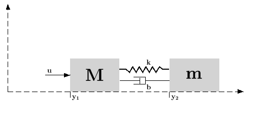
Assume the dynamical system formed by two masses connected by a spring and a damper:

A force $u=\bar{u}+e$ (where e is a noise) is applied to the big one. Here it is assumed that the deviations from equilibrium positions of the mass dy₁ and dy₂ positions has well as their derivatives are measured.

A state space representation of this system is:

$\dot{x}=\left[\begin{array}{llll}0&1&0&0\\ -k/M&-b/M&k/M&b/M\\ 0&0&0&1\\ k/m&b/m&-k/m&-b/m \end{array}\right] x +\left[\begin{array}{l}0\\ 1/M\\ 0\\ 0 \end{array}\right] u$

$\text{Where }x=\left[\begin{array}{l}dy_1\\ \dot{dy_1}\\ dy_2\\ \dot{dy_2}\end{array}\right]$

The LQ cost is defined by

$\int_0^\infty\left[\begin{array}{ll}x$

The following instructions may be used to compute a LQ compensator of this dynamical system.

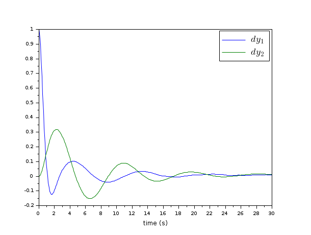
// Form the state space model (assume full state output)
M = 1; m = 0.2; k = 0.1; b = 0.004;
A = [  0     1    0    0
-k/M  -b/M  k/M  b/M
0     0    0    1
k/m  b/m  -k/m  -b/m];
B = [0; 1/M; 0; 0];
C = eye(4,4);
P = syslin("c",A, B, C);
//The compensator weights
Q_xx=diag([15 0 3 0]); //Weights on states
R_uu   = 0.5; //Weight on input
Kc=lqr(P,Q_xx,R_uu);

//form the Plant+compensator system

C=[1 0 0 0  //dy1
0 0 1 0];//dy2
S=C*(P/.(-Kc));
//check system stability
and(real(spec(S.A))<0)
// Check by simulation
dt=0.1;
t=0:dt:30;
u=0.1*rand(t);
y=csim(u,t,S,[1;0;0;0]);
clf;plot(t',y');xlabel(_("time (s)"))
L=legend(["$dy_1$","$dy_2$"]);L.font_size=4;

Reference

Engineering and Scientific Computing with Scilab, Claude Gomez and al.,Springer Science+Business Media, LLC,1999, ISNB:978-1-4612-7204-5

Report an issue
<< lqi	Linear Quadratic	Pole Placement >>

lqr