histplot
ヒストグラムをプロットする
呼び出し手順
histplot(n, data [,normalization] [,polygon], <opt_args>)
histplot(x, data [,normalization] [,polygon], <opt_args>)
cf = histplot(..)
引数
- n
正の整数 (クラスの数)
- x
クラスを定義する増加方向のベクトル (
xは2個以上の要素を有します)- data
ベクトル (解析するデータ)
- normalization
論理値 (%t (デフォルト値) または %f)
- polygon
論理値 (%t または %f (デフォルト値))
- <opt_args>
一連の命令
key1=value1,key2=value2,... を表します.ただし,key1,key2,...は任意のplot2d の オプションのパラメータ (style,strf,leg, rect,nax, logflag,frameflag, axesflag) とすることができます.- cf
これは一連の命令
key1=value1,key2=value2,...を表します. ただし,key1,key2,...は, plot2dの任意のオプションパラメータ (style,strf,leg, rect,nax, logflag,frameflag, axesflag) とすることができます.- cf
Computed frequencies (bins heighs)
説明
この関数は,クラスxを用いてdataベクトル
のヒストグラム(柱状グラフ)をプロットします.
xのかわりにクラスの数nが指令された場合,
クラスは等間隔でdx = (x(n+1)-x(1))/nとして
x(1) = min(data) < x(2) = x(1) + dx < ... < x(n+1) = max(data)
となるように選択されます.
クラスはC1 = [x(1), x(2)]およびi >= 2の時にCi = ( x(i), x(i+1)]
により定義されます.
dataの総数 Nmax (Nmax = length(data))となり,
Ciに含まれるdata要素の数 Niは
normalizationが true (デフォルト)の場合には
Ni/(Nmax (x(i+1)-x(i)))となります.
そうでない場合, Ni となります.
正規化が行われる場合,このヒストグラムは以下の制約を満たします:

任意の plot2d (オプション) パラメータを指定できます;
例えば,色番号2 (標準カラーマップを使用する場合には青)のヒストグラムをプロットする場合や,
矩形 [-3,3]x[0,0.5] の内側へのプロットを制限する場合,
histplot(n,data, style=2, rect=[-3,0,3,0.5])
を使用することができます.
周波数ポリゴンは,ヒストグラムの全てのビンの頂部の中点をつなぐことにより描画されるグラフn
線です.
このため, ポリゴン周波数チャートをプロットするために
histplot を使用できます.
オプションの引数 polygon は,直線を有するヒストグラムの
各バーの頂部の中点を接続します.
polygon=%tの場合,
周波数ポリゴンチャート付きのヒストグラムが出力されます.
デモを参照するには histplot()コマンドを入力してください.
例
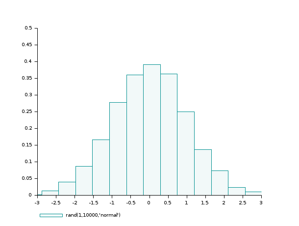
- 例 #1: ガウス乱数標本の種々のヒストグラム
d = rand(1,10000,'normal');  // ガウス乱数標本

clf(); histplot(20, d);
clf(); histplot(20, d, normalization=%f);
clf(); histplot(20, d, leg='rand(1,10000,''normal'')', style=5);
clf(); histplot(20, d, leg='rand(1,10000,''normal'')', style=16, rect=[-3,0,3,0.5]);
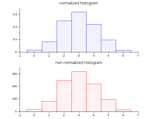
- 例 #2: 二項分布 (B(6,0.5)) 乱数標本のヒストグラム
d = grand(1000,1,"bin", 6, 0.5);
c = linspace(-0.5,6.5,8);

clf()
subplot(2,1,1)
histplot(c, d, style=2);
xtitle("normalized histogram")

subplot(2,1,2)
histplot(c, d, normalization=%f, style=5);
xtitle("non normalized histogram")
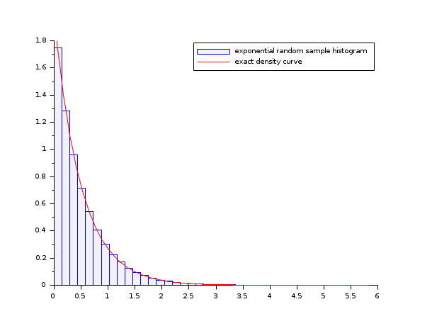
- 例 #3: 指数乱数標本のヒストグラム
lambda = 2;
X = grand(100000,1,"exp", 1/lambda);
Xmax = max(X);

clf()
histplot(40, X, style=2);
x = linspace(0,max(Xmax),100)';
plot2d(x,lambda*exp(-lambda*x),strf="000",style=5)
legend(["exponential random sample histogram" "exact density curve"]);
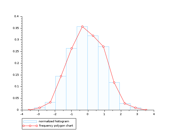
- 例 #4: 周波数ポリゴンチャートおよびガウス乱数標本のヒストグラム
n = 10;
data = rand(1,1000,"normal");

clf(); histplot(n, data, style=12, polygon=%t);
legend(["normalized histogram" "frequency polygon chart"],"lower_caption");
参照
履歴
| バージョン | 記述 |
| 5.5.0 | polygon option and cf output added. |
| Report an issue | ||
| << graypolarplot | 2d_plot | LineSpec >> |