- Scilabヘルプ
- Signal Processing
- filters
- analpf
- buttmag
- casc
- cheb1mag
- cheb2mag
- convol
- ell1mag
- eqfir
- eqiir
- faurre
- ffilt
- filter
- find_freq
- frmag
- fsfirlin
- group
- iir
- iirgroup
- iirlp
- kalm
- lev
- levin
- lindquist
- remez
- remezb
- srfaur
- srkf
- sskf
- syredi
- system
- trans
- wfir
- wiener
- wigner
- window
- yulewalk
- zpbutt
- zpch1
- zpch2
- zpell
Please note that the recommended version of Scilab is 2026.1.0. This page might be outdated.
See the recommended documentation of this function
window
様々な型の対称ウインドウを計算
呼び出し手順
win_l=window('re',n)

win_l=window('tr',n)

win_l=window('hn',n)

win_l=window('hm',n)

win_l=window('kr',n,Beta)

[win_l,cwp]=window('ch',n,par)
引数
- n
ウインドウの長さ
- par
2要素のベクトル
par=[dp,df])のパラメータで,dp(0<dp<.5) はメインローブの幅を規定し,dfはサイドローブの高さ (df>0)を規定します.これら2つの片方のみを指定することができ, もう片方には
-1を指定する必要があります.- Beta
カイザーウインドウのパラメータ
Beta >0).- win
ウインドウ
- cwp
未定義のチェビシェフウインドウのパラメータ
説明
デジタル信号処理用の様々な対称ウインドウを計算する関数です.
カイザーウインドウは,準最適ウインドウ関数です.
Betaは任意の正の実数で,ウインドウの形状を定義します. 整数nはウインドウの長さです.構築の際,この関数は,
k = n/2,すなわち,ウインドウの 中央,における最大値を 1 にし,ウインドウの端に向かって減少させます.Betaの大きさを大きくすると,ウインドはより狭くなります;Beta = 0の場合,矩形ウインドウと同じになります. 逆に,Betaを大きくすると,フーリエ変換における メインローブの幅が増加し,振幅のサイドローブは減少します. つまり,このパラメータはメインローブの幅とサイドローブの面積の トレードオフを制御します.Beta ウインドウ形状 0 矩形形状 5 ハミングウインドウを近似 6 ハニングウインドウを近似 8.6 ブラックマンウインドウを近似 チェビシェフウインドウは,指定した特定のサイドローブの高さのもとで, メインローブの幅を最小化します. このウインドウの特徴は,等リプル特性であり, 全てのサイドローブは同じ高さとなります.
ハニングおよびハミングウインドウは非常に似ており, パラメータ
Betaの選択のみが異なります:w=Beta+(1 - Beta)*cos(2*%pi*x/(n-1))Betaはハニングウインドでは 1/2 , ハミングウインドウでは 0.54 です.
例
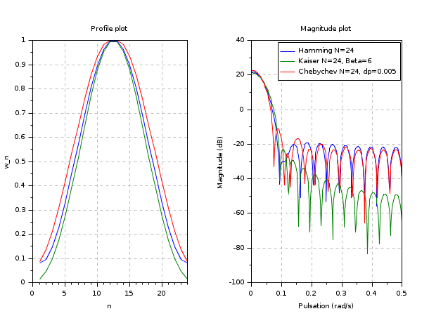
clf()
N=24;
whm=window('hm',N);//Hamming window
wkr=window('kr',N,6);//Hamming Kaiser window
wch=window('ch',N,[0.005,-1]);//Chebychev window
//plot the window profile
subplot(121);plot((1:N)',[whm;wkr;wch]')
set(gca(),'grid',[1 1]*color('gray'))
xlabel("n")
ylabel("w_n")
title(gettext("Profile plot"))
//plot the magnitude of the frequency responses
n=256;
[Whm,fr]=frmag(whm,n);
[Wkr,fr]=frmag(wkr,n);
[Wch,fr]=frmag(wch,n);
subplot(122);plot(fr',20*log10([Whm;Wkr;Wch]'))
set(gca(),'grid',[1 1]*color('gray'))
xlabel(gettext("Pulsation (rad/s)"))
ylabel(gettext("Magnitude (dB)"))
legend(["Hamming N=24";"Kaiser N=24, Beta=6";"Chebychev N=24, dp=0.005"]);
title(gettext("Magnitude plot"))
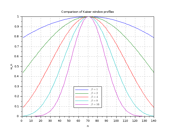
clf()
N=140;
w1=window('kr',N,1);
w2=window('kr',N,2);
w4=window('kr',N,4);
w8=window('kr',N,8);
w16=window('kr',N,16);

//plot the window profile
plot((1:N)',[w1;w2;w4;w8;w16]')
set(gca(),'grid',[1 1]*color('gray'))
legend("$\beta="+string([1;2;4;8;16])+'$',[55,0.3])
xlabel("n")
ylabel("w_n")
title(gettext("Comparison of Kaiser window profiles"))
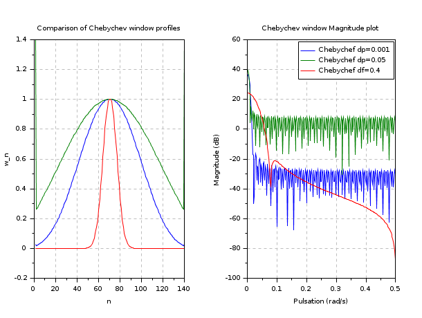
clf()
N=140;
w1=window('ch',N,[0.001,-1]);
w2=window('ch',N,[0.05,-1]);
w3=window('ch',N,[-1,0.4]);

//plot the window profile
subplot(121);plot((1:N)',[w1;w2;w3]')
set(gca(),'grid',[1 1]*color('gray'))
//legend("$\beta="+string([1;2;4;8;16])+'$',[55,0.3])
xlabel("n")
ylabel("w_n")
title(gettext("Comparison of Chebychev window profiles"))
//plot the magnitude of the frequency responses
n=256;
[W1,fr]=frmag(w1,n);
[W2,fr]=frmag(w2,n);
[W3,fr]=frmag(w3,n);
subplot(122);plot(fr',20*log10([W1;W2;W3]'))
set(gca(),'grid',[1 1]*color('gray'))
xlabel(gettext("Pulsation (rd/s)"))
ylabel(gettext("Magnitude (dB)"))
legend(["Chebychef dp=0.001";"Chebychef dp=0.05";"Chebychef df=0.4"]);
title(gettext("Chebychev window Magnitude plot"))
参考文献
IEEE. Programs for Digital Signal Processing. IEEE Press. New York: John Wiley and Sons, 1979. Program 5.2.
| Report an issue | ||
| << wigner | filters | yulewalk >> |