loglog
2D logarithmic plot
Syntax
loglog // demo
loglog(y)
loglog(x, y)
loglog(x, fun)
loglog(x, list(fun, param))
loglog(.., LineSpec)
loglog(.., LineSpec, GlobalProperty)
loglog(x1, y1, LineSpec1, x2,y2,LineSpec2,...xN, yN, LineSpecN, GlobalProperty1,.. GlobalPropertyM)
loglog(x1,fun1,LineSpec1, x2,y2,LineSpec2,...xN,funN,LineSpecN, GlobalProperty1, ..GlobalPropertyM)
loglog(axes_handle,...)
Arguments
- x
vector or matrix of strictly positive real numbers or integers. If omitted, it is assumed to be the vector
1:nwherenis the number of curve points given by theyparameter.- y
vector or matrix of strictly positive real numbers or integers.
- fun, fun1, ..
handle of a function, as in
loglog(x, gamma).If the function to plot needs some parameters as input arguments, the function and its parameters can be specified through a list, as in
loglog(x, list(delip, -0.4))- LineSpec
This optional argument must be a string that will be used as a shortcut to specify a way of drawing a line. We can have one
LineSpecperyor{x,y}previously entered.LineSpecoptions deals with LineStyle, Marker and Color specifiers (see LineSpec). Those specifiers determine the line style, mark style and color of the plotted lines.- GlobalProperty
This optional argument represents a sequence of couple statements
{PropertyName,PropertyValue}that defines global objects' properties applied to all the curves created by this plot. For a complete view of the available properties (see GlobalProperty).- axes_handle
This optional argument forces the plot to appear inside the selected axes given by
axes_handlerather than the current axes (see gca).
Description
loglog plots data using a base 10 logarithmic scale for both x-axis and y-axis. The possible syntaxes and arguments are the same as the plot function besides the condition that values in x and y arguments be strictly positive.
If the current axes is not empty and the x-axis or the y-axis has a negative lower bound then its scale will remain linear after the plot.
Enter the command loglog to see a demo.
Examples
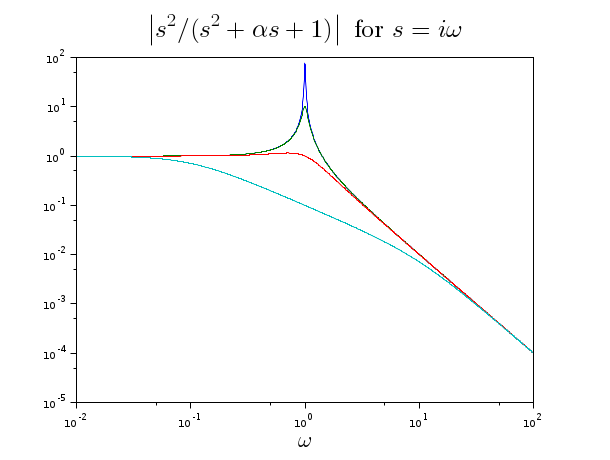
w=logspace(-2,2,1000);
s=%i*w;
g=[];
for alpha=logspace(-2,1,4);
  g=[g;(1)./(s.^2+alpha*s+1)];
end
clf("reset")

loglog(w,abs(g));

legend(leg)
title("$\LARGE \left|s^2/(s^2+\alpha s+1)\right|\mbox{ for }s=i\omega$")
xlabel("$\LARGE \omega$")
See also
- plot — 2D plot
- semilogx — 2D semilogarithmic plot
- semilogy — 2D semilogarithmic plot
- LineSpec — to quickly customize the lines appearance in a plot
- GlobalProperty — customizes the objects appearance (curves, surfaces...) in a plot or surf command
History
| Version | Description |
| 6.1.1 | Function loglog added. |
| Report an issue | ||
| << histplot | 2d_plot | paramfplot2d >> |