Complex solutions
Computing a complex solution and its applications
Basic complex solution
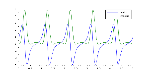
Unlike the native implementation, the SUNDIALS solvers Scilab interface allows to solve a system of equations, ODEs or DAEs if the solution is complex, when the user functions (right hand side or residual, Jacobian) are given by Scilab functions. For example, for an ODE, the solution is complex when the right hand side always yields complex values or when the initial condition is complex, even if the right hand side is a real function. Here is a basic example:
function out=crhs(t, y)
    out = 10*exp(2*%i*%pi*t)*y;
endfunction
[t,z] = cvode(crhs,[0 5],1);
plot(t,real(z),t,imag(z))
legend("real(z)","imag(z)");
Sensitivity computation with complex step
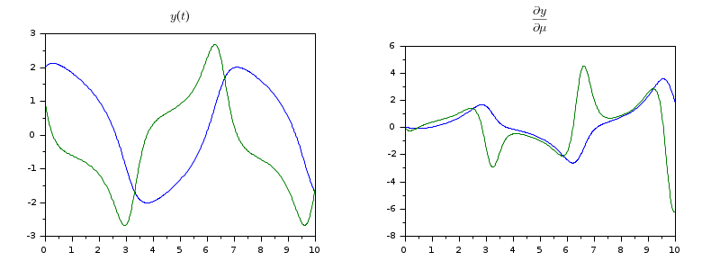
Computing the sensitivity function of the solution with respect to a parameter, on the whole integration interval or just at given time points is typically used when you need to solve identification problems where the model involves an ODE or a DAE. Using the complex step technique allows to compute, up to machine precision, the derivative of the solution with respect to a chosen parameter, which can appear in the computation of the right hand side or in the initial condition, and more generally, a directional derivative. The cvode and ida solvers already includes a built in feature (see the ODE Sensitivity and DAE Sensitivity help pages) that allows to compute the sensitivity function by adding its derivative (user provided or approximated with finite difference quotients) to the original ODE rhs or DAE residual. However, when such a feature is not available (for example with arkode) and when the rhs is computed by a Scilab function, the sensititivity with respect to a single parameter can be computed by using a complex step. In the following example, we compute the derivative of the solution of the Van Der Pol equation with respect to mu. Note that the real part of the complex solution gives the solution of the equation itself:
function dydt=vdp(t, y, mu)
    dydt = [y(2,:)
            mu*(1-y(1,:).*y(1,:)).*y(2,:)-y(1,:)];
endfunction
y0=[2;1];
h = 1e-200;
mu = 1;
[t,yc] = arkode(list(vdp,complex(mu,h)), [0,10], y0);
dydmu = imag(yc)/h;
y = real(yc);
subplot(1,2,1)
title("$$y(t)$$")
plot(t,y)
subplot(1,2,2)
plot(t,dydmu)
title("$$\frac{\partial y}{\partial \mu}(t,y)$$")
See also
- arkode — SUNDIALS ordinary differential equation additive Runge-Kutta solver
- cvode — SUNDIALS ordinary differential equation solver
- ida — SUNDIALS differential-algebraic equation solver
- kinsol — SUNDIALS general-purpose nonlinear system solver
- ODE Sensitivity — Forward Sensitivity computation with cvode
- DAE Sensitivity — Forward Sensitivity computation with ida
Bibliography
Al-Mohy, A.H., Higham, N.J. The complex step approximation to the Fréchet derivative of a matrix function. Numer Algor 53, 133 (2010). https://doi.org/10.1007/s11075-009-9323-y
| Report an issue | ||
| << Callback | Options, features and user functions | Events >> |