arkode
SUNDIALS ordinary differential equation additive Runge-Kutta solver
Syntax
[t,y] = arkode(f,tspan,y0,options)
[t,y,info] = arkode(f,tspan,y0,options)
sol = arkode(...)
solext = arkode(sol,tfinal,options)
arkode(...)
Arguments
| f | a function, a string or a list, the right hand side of the differential equation |
| tspan | double vector, time interval or time points |
| y0 | a double array: initial state of the ode |
| options | a sequence of optional named arguments, see the solvers options |
| t | vector of time points used by the solver |
| y | array of solution at time values in t |
| sol, solext | MList of |
| info | MList of |
| tfinal | final time of extended solution |
Description
arkode computes the solution of real or complex ordinary different equations defined by

The right hand side can be specfied as the sum of two functions  where
where
 is typically stiff and needs to be integrated by an implicit method, whereas
 is the non-stiff part of
  . When both components are specified
arkode uses an implicit/explicit method (see the dedicated section below).
When the splitting is not necessary a classical explicit (the default) or implicit method can be used
(see the available methods below).
The mass matrix M(t) is by default the identity matrix. It can be changed to any non-singular matrix by giving a constant
matrix to the mass option or a user function if the matrix is time-dependent. See the
mass matrix section below). If the mass matrix depends on solution y then the problem
has to be reformulated as a DAE and can be solved by ida.
As arkode shares with cvode most of its features (syntax, specification of user function) please refer to the Description section of cvode help page for basic usage (events handling, solution output, callback). We will give below an example where the solution is computed first with the default explicit method, then with an implicit/explicit method.
Example
In the following example, we solve the Brusselator ODE

The right hand side is computed by the function %SUN_bruss (already defined in the SUNDIALS module):
function dydt=%SUN_bruss(t, y, a, b, ep)
u=y(1); v=y(2); w=y(3);
dydt = [a-(w+1)*u+v*u*u; w*u-v*u*u; (b-w)/ep-w*u];
end
u0 = 3.9; v0 = 1.1; w0 = 2.8; a  = 1.2; b  = 2.5; ep = 1.0e-1;
[t,y] = arkode(list(%SUN_bruss,a,b,ep), [0 10], [u0; v0; w0]);
plot(t,y)
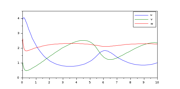
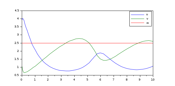
In the example above the default explicit order 4 Runge-Kutta method is used. However, when
a very small value is taken for  an implicit scheme can be used, here the default order 4
diagonaly implicit Runge-Kutta method:
an implicit scheme can be used, here the default order 4
diagonaly implicit Runge-Kutta method:
u0 = 3.9; v0 = 1.1; w0 = 2.8; a  = 1.2; b  = 2.5; ep = 1.0e-5;
[t,y] = arkode(list(%SUN_bruss,a,b,ep), [0 10], [u0; v0; w0], method="DIRK");
plot(t,y)
Using an implicit/explicit method
In the above example we can split the right hand side in two components like this :
function dydt=%SUN_brussI(t, y, b, ep)
    w=y(3);
    dydt = [0; 0; (b-w)/ep];
end
function dydt=%SUN_brussE(t, y, a)
    u=y(1); v=y(2); w=y(3);
    dydt = [a-(w+1)*u+v*u*u; w*u-v*u*u;-w*u];
end
and solve the differential equation with the default order 4 implicit/explicit method. The solver just needs the information about the splitting,
which is given by the stiffRhs option:
u0 = 3.9; v0 = 1.1; w0 = 2.8; a  = 1.2; b  = 2.5; ep = 1.0e-5;
jacI = [0 0 0;0 0 0;0 0 -1/ep];
[t,y] = arkode(list(%SUN_brussE,a), [0 10], [u0; v0; w0], stiffRhs = list(%SUN_brussI,b,ep), ...
               jacobian = jacI);
plot(t,y)
This small example exhibits the interest of the splitting because here the stiff component is linear and we can specify its constant Jacobian to improve the performance of the inner implicit method. Note that when using an ImEx method with a user-provided Jacobian, the latter is the Jacobian of the stiff component only.
Mass matrix
When using arkode a non singular mass matrix can be specified and to this purpose the call to the solver takes the form
arkode(f,tspan,y0,mass=massFun) where
massFun can be:
a function with prototype
m=massFun(t), for example:function m=massFun(t) m = [1 0;0 1+t] end [t,y] = arkode(%SUN_vdp1, [0 10], [0; 2], mass = massFun);
a matrix, which allows inform the solver that the mass does not depend on time:
[t,y] = arkode(%SUN_vdp1, [0 10], [0; 2], mass = [1 0;0 2]);
a string giving the name of a SUNDIALS DLL entrypoint with C prototype
int sunMass(realtype t, SUNMatrix M, void* user_data, N_Vector tmp1,
                                      N_Vector tmp2, N_Vector tmp3)
code=[
    "#include <nvector/nvector_serial.h>"
    "#include <sunmatrix/sunmatrix_dense.h>"
    "int sunRhs(realtype t, N_Vector Y, N_Vector Yd, void *user_data)"
    "{"
    "double *y = NV_DATA_S(Y);"
    "double *ydot = NV_DATA_S(Yd);"
    "ydot[0] = y[1];"
    "ydot[1] = (1-y[0]*y[0])*y[1]-y[0];"
    "return 0;"
    "}"
    "int sunMass(realtype t, SUNMatrix M, void* user_data, N_Vector tmp1,"
    "            N_Vector tmp2, N_Vector tmp3)"
    "{"
    "double *mass = SM_DATA_D(M);"
    "mass[0] = 1.0; mass[1] = 0.0;"
    "mass[2] = 0.0;  mass[3]= 1.0+t;"
    "return 0;"
    "}"];
mputl(code,"code.c")
SUN_Clink(["sunRhs","sunMass"],"code.c",load=%t);
[t1,y1]=arkode("sunRhs",[0 10],[2;1],mass="sunMass");
Available arkode methods
When there is no additive splitting of the right hand side the default method is the order 4 explicit Zonneveld method (identifiers ERK, ERK_4 or ZONNEVELD_5_3_4). An implicit method can be chosen by using the method option. Note that adding a user Jacobian automatically selects the default implicit method.
If splitting of the right hand side is necessary and the stiff component is given with the stiffRhs option, the default method is a combined order 4 implicit/explicit method (ARK436L2SA_DIRK_6_3_4 and ARK436L2SA_ERK_6_3_4) with identifier ARK or ARK_4.
If you need a custom ERK, DIRK or ARK method see the next section.
| Method identifier | Kind | Order | Aliases |
| HEUN_EULER_2_1_2 | explicit | 2 | ERK_2 |
| BOGACKI_SHAMPINE_4_2_3 | explicit | 3 | ERK_3 |
| ARK324L2SA_ERK_4_2_3 | explicit | 3 | |
| ZONNEVELD_5_3_4 | explicit | 4 | ERK, ERK_4 |
| ARK436L2SA_ERK_6_3_4 | explicit | 4 | |
| SAYFY_ABURUB_6_3_4 | explicit | 4 | |
| ARK437L2SA_ERK_7_3_4 | explicit | 4 | |
| CASH_KARP_6_4_5 | explicit | 5 | ERK_5 |
| FEHLBERG_6_4_5 | explicit | 5 | |
| ARK548L2SA_ERK_8_4_5 | explicit | 5 | |
| ARK548L2SAb_ERK_8_4_5 | explicit | 5 | |
| VERNER_8_5_6 | explicit | 6 | ERK_6 |
| FEHLBERG_13_7_8 | explicit | 8 | ERK_8 |
| SDIRK_2_1_2 | implicit | 2 | DIRK_2 |
| BILLINGTON_3_3_2 | implicit | 2 | |
| TRBDF2_3_3_2 | implicit | 2 | |
| KVAERNO_4_2_3 | implicit | 3 | |
| ESDIRK324L2SA_4_2_3 | implicit | 3 | |
| ESDIRK325L2SA_5_2_3 | implicit | 3 | |
| ESDIRK32I5L2SA_5_2_3 | implicit | 3 | |
| ARK324L2SA_DIRK_4_2_3 | implicit | 3 | DIRK_3 |
| CASH_5_2_4 | implicit | 4 | |
| KVAERNO_5_3_4 | implicit | 4 | |
| CASH_5_2_4 | implicit | 4 | |
| CASH_5_3_4 | implicit | 4 | |
| SDIRK_5_3_4 | implicit | 4 | DIRK, DIRK_4 |
| KVAERNO_5_3_4 | implicit | 4 | |
| ARK436L2SA_DIRK_6_3_4 | implicit | 4 | |
| ARK437L2SA_DIRK_7_3_4 | implicit | 4 | |
| ESDIRK436L2SA_6_3_4 | implicit | 4 | |
| ESDIRK43I6L2SA_6_3_4 | implicit | 4 | |
| QESDIRK436L2SA_6_3_4 | implicit | 4 | |
| ESDIRK437L2SA_7_3_4 | implicit | 4 | |
| KVAERNO_7_4_5 | implicit | 5 | |
| ARK548L2SA_DIRK_8_4_5 | implicit | 5 | DIRK_5 |
| ARK548L2SAb_DIRK_8_4_5 | implicit | 5 | |
| ESDIRK547L2SA_7_4_5 | implicit | 5 | |
| ESDIRK547L2SA2_7_4_5 | implicit | 5 | |
| ARK324 | imex | 3 | ARK_3 |
| ARK436 | imex | 4 | ARK, ARK_4 |
| ARK437 | imex | 4 | |
| ARK548 | imex | 5 | ARK_5 |
| ARK548b | imex | 5 |
Using custom Butcher tableaux
The ERKButcherTab and/or DIRKButcherTab options allow to specify custom Butcher tableaux, under the form of a matrix of size (s+2,s+1) or (s+1,s+1) where s is the number of stages of the method :

A is a matrix of size (s,s), c a column vector of length s, b and d are row vectors of length s, the coefficients of the main and the embedded method,
of respective orders q and p. When there is no embedded method (above matrix on the right) the overall matrix has size (s+1,s+1) and
adaptive stepping is disabled, hence the option fixedStep must be set to the value of the chosen fixed step. Please note that
with a fixed step no error control occurs hence the computed solution may be very inaccurate.
The claimed orders and the structure of A are checked before initialization of the solver: only explicit or diagonally implicit methods are accepted (although the order check allows fully implicit methods). Both options can be used to build a custom additive imEx method, in that case the overall method order can be less than individual ERK/DIRK methods and can be checked in the the arkode solution output.
The explicit Euler and implicit Euler method with fixed step (mandatory in that case) can be specified by:
s1 = arkode(%SUN_vdp1,[0 1],[2;1],ERKButcherTab=[0 0;1 1],fixedStep=0.01);
s2 = arkode(%SUN_vdp1,[0 1],[2;1],DIRKButcherTab=[1 1;1 1],fixedStep=0.01);
The embedded explicit Heun-Euler method can be specified like this,
A = [0 0; 1 0];
c = [0; 1];
b = [0.5 0.5];
d = [1 0];
q = 2;
p = 1;
s = arkode(%SUN_vdp1,[0 10],[2;1],ERKButcherTab=[c A;q b;p d]);
and the implicit trapezoidal rule with implicit Euler embedding has the following tableau
A = [1 0; -1 1];
c = [1; 0];
b = [0.5 0.5];
d = [1 0];
q = 2;
p = 1;
s = arkode(%SUN_vdp1,[0 10],[2;1],DIRKButcherTab=[c A;q b;p d]);
The SUNDIALS module also provides functions %SUN_Tsitouras5,
%SUN_DormandPrince6 and %SUN_DormandPrince8 yielding classical tableaux (see references below):
s1 = arkode(%SUN_vdp1,[0 10],[2;1],ERKButcherTab = %SUN_Tsitouras5());
s2 = arkode(%SUN_vdp1,[0 10],[2;1],ERKButcherTab = %SUN_DormandPrince6());
s3 = arkode(%SUN_vdp1,[0 10],[2;1],ERKButcherTab = %SUN_DormandPrince8());
See also
- cvode — SUNDIALS ordinary differential equation solver
- ida — SUNDIALS differential-algebraic equation solver
- User functions — Coding user functions used by SUNDIALS solvers
- Options (ODE and DAE solvers) — Changing the default behavior of solver
Bibliography
A. C. Hindmarsh, P. N. Brown, K. E. Grant, S. L. Lee, R. Serban, D. E. Shumaker, and C. S. Woodward, "SUNDIALS: Suite of Nonlinear and Differential/Algebraic Equation Solvers," ACM Transactions on Mathematical Software, 31(3), pp. 363-396, 2005. Also available as LLNL technical report UCRL-JP-200037.
Daniel R. Reynolds and David J. Gardner and Carol S. Woodward and Cody J. Balos, "User Documentation for arkode", 2021, v5.1.1, available online at https://sundials.readthedocs.io/en/latest/arkode.
P.J. Prince and J. R. Dormand, High order embedded Runge-Kutta formulae, Journal of Computational and Applied Mathematics, 7 (1981), pp. 67-75.
Ch. Tsitouras, Runge–Kutta pairs of order 5(4) satisfying only the first column simplifying assumption, Computers & Mathematics with Applications, Volume 62, Issue 2, 2011, Pages 770-775, ISSN 0898-1221, https://doi.org/10.1016/j.camwa.2011.06.002.
| Report an issue | ||
| << Options, features and user functions | SUite of Nonlinear and DIfferential/ALgebraic equation - SUNDIALS solvers | cvode >> |