cvode
SUNDIALS ordinary differential equation solver
Syntax
[t,y] = cvode(f,tspan,y0,options)
[t,y,info] = cvode(f,tspan,y0,options)
sol = cvode(...)
solext = cvode(sol,tfinal,options)
cvode(...)
Arguments
| f | a function, a string or a list, the right hand side of the differential equation |
| tspan | double vector, time interval or time points |
| y0 | a double array: initial state of the ode |
| options | a sequence of optional named arguments, see the solvers options |
| t | vector of time points used by the solver |
| y | array of solution at time values in t |
| sol, solext | MList of |
| info | MList of |
| tfinal | final time of extended solution |
Description
cvode computes the solution of real or complex ordinary different equations defined by

It is an interface to the cvodes solver of SUNDIALS library with default ADAMS method (BDF method can be chosen in options). The solver has a specific feature which allows to compute the sensitivity with respect to a vector of parameters present in the initial condition and/or the right hand side (see the ODE Sensitivity dedicated help page).
The solver can also keep the solution in a given constraint manifold by projection (see the dedicated section below).
In addition, unlike the native SUNDIALS implementation, the Scilab interface allows to solve an ODE when the solution
is complex (see the
Complex ODE and DAE). Note: the description below is also valid for the arkode solver (except
the projection feature and sensitivity computation).
In its simplest form, the solver call takes the form
[t,y] = cvode(f,[t0 tf],y0)
where y0 is the
initial condition, t0, tf are the initial and final time, y is the
array of solution values [y(t(1)),y(t(2)),...] at time values in t, where concatenation is done on
next dimension if y0 is not a column vector (e.g. a matrix with at least 2 columns). The time values in t
are those used by the solver to meet default relative and absolute estimated local error (which can be changed in options).
In the simplest case the right hand side is computed by a Scilab function with two arguments, for example for the ode  the right hand side is coded as
function yprime=f(t, y)
    yprime = t+y
end
See the User functions help page to learn how to pass extra parameters and/or use DLL entrypoints.
When t has more than two components:
[t,y] = cvode(f,[t0 t1 ... tf],y0)
the solution is computed at prescribed points with the same precision as the two components syntax. However, the result may slightly differ
(within chosen tolerance) since t1-t0 may give a different guess of the initial step used by the solver. Provided
that the initial step is the same, further solver internal steps will be the same and solution at intermediate user points is computed by
continuous extension (native interpolation) formulas.
When searching for  where some functions defined in
 options vanish
(see the Events help page) the syntax
[t,y,te,ye,ie] = cvode(f,tspan,y0,options)
allows to recover  values in
 info.te, info.ye, info.ype and in info.ie the number(s) of the vanishing function.
When solution has to be further evaluated at arbitrary points which are not known in advance, then the syntax
sol = cvode(f,[t0 tf],y0)
yields an MList of _odeSolution type, which can be used later as an interpolant, see the
Solution output help page.
When no ouput argument is given, the only way to have access to the solution at solver or user time steps is to use a user callback (see the User functions help page). For example, when there could be memory issues (e.g. if the dimension of the solution vector is very large) this allows to write the solution to disk.
Example
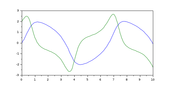
In the following example, we solve the Ordinary Differential Equation
 with the initial
condition
with the initial
condition  and
and  . Since the original equation is of second order
we define the state of the equivalent first order equation as
. Since the original equation is of second order
we define the state of the equivalent first order equation as  . The right hand side is computed by the
function
. The right hand side is computed by the
function %SUN_vdp1 (defined in the SUNDIALS module):
function vdot=%SUN_vdp1(t, v)
    mu = 1;
    vdot = [v(2); mu*(1-v(1)^2)*v(2)-v(1)]
end
[t,v] = cvode(%SUN_vdp1, [0 10], [0; 2]);
plot(t,v)
Projection on a constraint manifold
cvode can solve initial value problems of the kind

where the initial condition is supposed to verify the constraint. Instead of the contraint function g(t,y),
the user has to provide a projection function given as a Scilab function or a SUNDIALS DLL to the
projection option. The call to cvode takes the form
cvode(f, tspan, y0, projection = projFun, projectError = b)
When using a Scilab function, projFun has the prototype
[corr, err] = projFun(t,y,err) and b is a boolean.
The function has to yield in corr the difference
between y and its projection (orthogonal or other) on the constraint manifold, i.e.
corr is such that y+corr
satisfies the constraint equation. When b is true then the function should
also yield the projection of the error vector err.
When the option projectError is not set, err
is passed as an empty matrix. Here is an example for a particle moving conterclockwise with velocity alpha
on the unit circle in the xy-plane, where the solution is computed without and with projection:
function Xd=f(t, X, alpha)
    Xd = alpha*[-X(2);X(1)];
end
function corr=proj(t, X, err)
    corr = X/norm(X) - X;
end

alpha = 1;
X0 = [1;0];
tspan = 0:5;

[t,X]=cvode(list(f,alpha), tspan, X0,jacobian=[0 -alpha, alpha 0]);
disp(X-[cos(t);sin(t)])
disp(sum(X.^2,1))

[t,X]=cvode(list(f,alpha), tspan, X0,jacobian=[0 -alpha, alpha 0],projection=proj);
disp(X-[cos(t);sin(t)])
disp(sum(X.^2,1))
When the projection function is a DLL entry point, it must have the prototype
int sunProj(realtype t, N_Vector X, N_Vector Corr, realtype epsProj, N_Vector Err,
void *user_data)
When the err pointer is not NULL then projection of the error has to be done. The epsProj
input argument gives the actual value of the tolerance used in the nonlinear solver stopping test when solving the
nonlinear constrainted least squares problem (it cannot be changed by the projection function). Here is an example:
code=[
"#include <math.h>"
"#include <nvector/nvector_serial.h>"
"int sunRhs(realtype t, N_Vector X, N_Vector Xd, void *user_data)"
"{"
"double *x = NV_DATA_S(X);"
"double *xd = NV_DATA_S(Xd);"
"double *alpha = (double *)user_data;"
"xd[0] = -alpha[0]*x[1];"
"xd[1] = alpha[0]*x[0];"
"return 0;"
"}"
"int sunProj(realtype t, N_Vector X, N_Vector Corr, realtype epsProj, N_Vector Err, "
"            void *user_data)"
"{"
"double *x = NV_DATA_S(X);"
"double *corr = NV_DATA_S(Corr);"
"double R = sqrt(x[0]*x[0]+x[1]*x[1]);"
"corr[0] = x[0]/R-x[0];"
"corr[1] = x[1]/R-x[1];"
"return 0;"
"}"]
mputl(code,"code.c")
SUN_Clink(["sunRhs","sunProj"],"code.c",load=%t);
[t,x] = cvode(list("sunRhs",1),[0 10],[1 0],projection="sunProj");
sum(x.^2,1)
Sensitivity computation
cvode can solve initial value problems of the kind

where the sensitivity function is  . The right hand side of the sensitivity equation can be provided
by the user (see the
. The right hand side of the sensitivity equation can be provided
by the user (see the sensRhs option in the ODE Sensitivtiy help page) but by default the directional
derivatives are approximated by finite differences. The call to cvode takes the form
cvode(fun, tspan, y0, sensPar = p)
When using a Scilab function, fun has the prototype dydt = fun(t,y,p,...). Here is an example
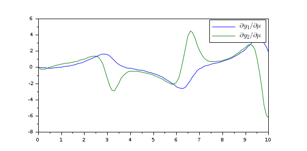
where we compute the sensitivity of the solution of the Van Der Pol equation with respect to parameter mu:
function vdot=vdp(t, y, μ)
    vdot = [y(2); μ*(1-y(1)^2)*y(2)-y(1)]
end
[t,y,info] = cvode(vdp, 0:0.1:10, [2;1], sensPar = 1);
plot(t,info.s)
legend("$\Large\partial y_"+["1","2"]+"/\partial μ$");
Several options are available, see the ODE Sensitivity help page.
See also
- ODE Sensitivity — Forward Sensitivity computation with cvode
- arkode — SUNDIALS ordinary differential equation additive Runge-Kutta solver
- ida — SUNDIALS differential-algebraic equation solver
- User functions — Coding user functions used by SUNDIALS solvers
- Options (ODE and DAE solvers) — Changing the default behavior of solver
Bibliography
A. C. Hindmarsh, P. N. Brown, K. E. Grant, S. L. Lee, R. Serban, D. E. Shumaker, and C. S. Woodward, "SUNDIALS: Suite of Nonlinear and Differential/Algebraic Equation Solvers," ACM Transactions on Mathematical Software, 31(3), pp. 363-396, 2005. Also available as LLNL technical report UCRL-JP-200037.
Alan C. Hindmarsh, Radu Serban, Cody J. Balos, David J. Gardner, Daniel R. Reynolds, and Carol S. Woodward, "User Documentation for cvodeS", 2021, v6.1.1, available online at https://sundials.readthedocs.io/en/latest/cvodes.
| Report an issue | ||
| << arkode | SUite of Nonlinear and DIfferential/ALgebraic equation - SUNDIALS solvers | ida >> |