Sensitivity (ODE)
Forward Sensitivity computation with cvode
Syntax
[t,y,info] = cvode(f,tspan,y0, sensPar = pvalue, options)
sol = cvode( ... , sensPar = pvalue, options)
Arguments
| pvalue | a real double array: the value of parameters with respect to which sensitivity is computed |
| options | a sequence of optional named arguments (see the solvers options) and below for sensitivity specific options. |
| t | vector of time points used by the solver. |
| y | array of solution at time values in t |
| info | MList of |
| sol | MList of |
Description
While integrating an ODE where the right hand side f(t,y,p) depends on a vector p of parameters, cvode can compute simultaneously the
solution vector y at given time points and also  the derivative of the solution with
respect to p, i.e. the sensitivity matrix/function.
This amounts to augment the original ODE with the sensitivity equation, which is obtained by formal derivation of the original ODE
with respect to p:
the derivative of the solution with
respect to p, i.e. the sensitivity matrix/function.
This amounts to augment the original ODE with the sensitivity equation, which is obtained by formal derivation of the original ODE
with respect to p:

The sensitivity matrix is typically used when solving identification parameter problems, for example nonlinear regression, and it can serve both aspects of the problem solution, i.e. qualitative and quantitative: studying the sensitivity on the time span can help to state identifiability of the parameters whereas computing the sensitivity at precise time points of measurements allows to compute the gradient of the squared norm of the residual.
When the right hand side of the ODE is
explicitely known then the right hand side of the sensitivity equation can be provided (see the sensRhs below), but cvode can also
approximate it by approximating directional derivatives by finite difference quotients.
The sensitivity computation is triggered by using the sensPar option:
where the sensitivity of the solution is retrieved in the "s" field of either the info or sol output argument.
When the right hand side of the ODE is yielded by a Scilab function, the protoype of fun must include a formal
input argument after the regular (t,y) pair (denoted p below), which will contain the parameter values. Additionnal user parameters
must be given as explained in the User functions help page :
dydt = fun(t, y, p, ...)
When the right hand side of the ODE is yielded by a DLL entry point, as only one array of double values can be passed,
complimentary user parameters must be passed together with sensitivity parameters in the same vector. The actual sensitivity
parameters can be precised by using the sensParIndex (see below).
Note that the yielded s array has dimensions (length(y0), length(p), length(t)) but singleton dimensions are squeezed when p or the ODE state is a scalar. The sensitivity related output arguments s and se can also be recovered in the solution output as complimentary fields.
Example
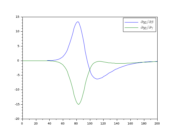
Here we compute the sensitivity of the solution of the SIR epidemiologic system with respect to initial value y2(0), parameters β, γ and
plot only the sensitivity of y(2) with respect to β and γ. Option yS0 allows to give the initial value of the sensitivity.
function dydt=sir(t, y, p)
    β = p(2);
    γ = p(3);
    dydt = [-β*y(1)*y(2)
             β*y(1)*y(2)-γ*y(2)
             γ*y(2)];
end
y20 = 1e-6;
β = 0.2;
γ = 0.05;
y0 = [1-y20; y20; 0];
[t,y,info] = cvode(sir, [0 200], y0, sensPar = [y20;β;γ], yS0 = [-1 0 0 ;1 0 0;0 0 0], method="BDF");
plot(t',squeeze(info.s(2,2:3,:))')
legend("$\Large\partial y_2/\partial"+["\beta","\gamma"]+"$");
Options
| sensPar | a double array with the values of parameters w.r.t. which sensitivity is to be computed. |
| sensParIndex | an array of integers between 1 and function dydt=sir(t, y, p) β = p(2); γ = p(3); dydt = [-β*y(1)*y(2) β*y(1)*y(2)-γ*y(2) γ*y(2)]; end y20 = 1e-6; β = 0.2; γ = 0.05; y0 = [1-y20; y20; 0]; [t,y,info]=cvode(sir, [0 200], y0, sensPar=[y20;β;γ], sensParIndex=2, method="BDF"); plot(t',info.s') legend("$\Large\partial y_"+["1","2","3"]+"/\partial \beta$"); 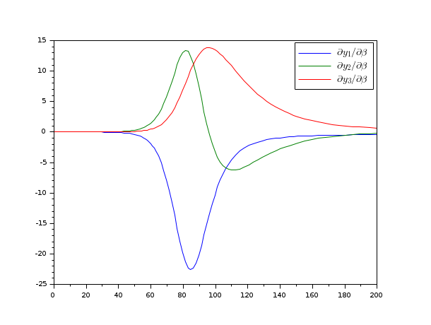 |
| yS0 | The initial condition of the sensitivity function, i.e. |
| sensRhs | a function, a string or a list, the right hand side of the sensitivity function. When the right hand side of the ODE is known explicitely and computation of its derivative is tractable (e.g. by symbolic differentiation or by any automatic procedure, including complex step), giving the true rhs of the sensitivity function improves the precision and the computation time. When sensRhs is a Scilab function, its prototype must be dsdt = sensRhs(t, y, s, p, ...) In the following example, the sensParIndex is only used to guess the number of actual sensitivity parameters (here only beta) when they are not all considered: function dydt=sir(t, y, p) β = p(2); γ = p(3); dydt = [-β*y(1)*y(2) β*y(1)*y(2)-γ*y(2) γ*y(2)]; end function dsdt=sirSens(t, y, s, p) β = p(2); γ = p(3); ds1dt = -β*(y(2)*s(1)+y(1)*s(2))-y(1)*y(2); dsdt = [ ds1dt; -ds1dt-γ*s(2); γ*s(2)] end y20 = 1e-6; β = 0.2; γ = 0.05; y0 = [1-y20; y20; 0]; [t,y,info]=cvode(sir, [0 200], y0, sensPar=[y20;β;γ], sensParIndex=2, sensRhs=sirSens, method="BDF"); plot(t,info.s) legend("$\Large\partial y_"+["1","2","3"]+"/\partial \beta$"); |
| sensErrCon | By default, sensErrCon is set to %f. If sensErrCon=%t then both state variables and sensitivity variables are included in the error tests. |
| sensCorrStep | "simultaneous" (the default) or "staggered": when sensCorrStep="simultaneous", the state and sensitivity variables are corrected at the same time. If sensCorrStep="staggered", the correction step for the sensitivity variables takes place at the same time for all sensitivity equations, but only after the correction of the state variables has converged and the state variables have passed the local error test. |
| typicalPar | This option serves as positive scaling factors when the right-hand side of the sensitivity is computed by cvode using internal finite difference-quotients. The results will be more accurate if an order of magnitude information is provided. Typically, if no component vanishes, the value of sensPar can be used. |

See also
- arkode — SUNDIALS ordinary differential equation additive Runge-Kutta solver
- cvode — SUNDIALS ordinary differential equation solver
- ida — SUNDIALS differential-algebraic equation solver
- DAE Sensitivity — Forward Sensitivity computation with ida
- User functions — Coding user functions used by SUNDIALS solvers
- Options (ODE and DAE solvers) — Changing the default behavior of solver
- SUN_Clink — Compiling and linking a C user function
| Report an issue | ||
| << Sensitivity (DAE) | Options, features and user functions | Solution output (ODE and DAE solvers) >> |