Please note that the recommended version of Scilab is 2026.1.0. This page might be outdated.
See the recommended documentation of this function
CLSS
Continuous state-space system
Block Screenshot
Contents
Description
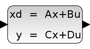
This block realizes a continuous-time linear state-space system.

where x is the vector of state variables, u is the vector of input functions and y is the vector of output variables.
The system is defined by the (A, B, C, D) matrices and the initial state X0. The dimensions must be compatible.
Parameters
A matrix
A square matrix.
Properties : Type 'mat' of size [-1,-1].
B matrix
The B matrix, [] if system has no input.
Properties : Type 'mat' of size ["size(%1,2)","-1"].
C matrix
The C matrix , [] if system has no output.
Properties : Type 'mat' of size ["-1","size(%1,2)"].
D matrix
The D matrix, [] if system has no D term.
Properties : Type 'mat' of size [-1,-1].
Initial state
A vector/scalar initial state of the system.
Properties : Type 'vec' of size "size(%1,2)".
Default properties
always active: yes
direct-feedthrough: no
zero-crossing: no
mode: no
regular inputs:
- port 1 : size [1,1] / type 1
regular outputs:
- port 1 : size [1,1] / type 1
number/sizes of activation inputs: 0
number/sizes of activation outputs: 0
continuous-time state: yes
discrete-time state: no
object discrete-time state: no
name of computational function: csslti4
Interfacing function
SCI/modules/scicos_blocks/macros/Linear/CLSS.sci
Computational function
SCI/modules/scicos_blocks/src/c/csslti4.c (Type 4)
Example
This sample example illustrates how to use CLSS block to simulate and display the output waveform y(t)=Vc(t) of the RLC circuit shown below.
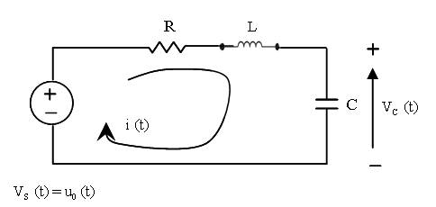
The equations for an RLC circuit are the following. They result from Kirchhoff's voltage law and Newton's law.

The R, L and C are the system's resistance, inductance and capacitor.
We define the capacitor voltage Vc and the
inductance current iL as the state variables
X1 and X2.

thus

Rearranging these equations we get:

These equations can be put into matrix form as follows,

The required output equation is

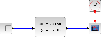
The following diagram shows these equations modeled in Xcos where R= 10 Ω, L= 5 mΗ and C= 0.1 µF; the initial states are x1=0 and x2=0.5.
To obtain the output Vc(t) we use CLSS block from Continuous time systems Palette.

| Report an issue | ||
| << CLR | Continuous_pal | DERIV >> |