Scilab 6.1.0
- Scilab Help
- Signal Processing
- Filters
- How to design an elliptic filter
- analpf
- buttmag
- casc
- cheb1mag
- cheb2mag
- ell1mag
- eqfir
- eqiir
- faurre
- ffilt
- filt_sinc
- filter
- find_freq
- frmag
- fsfirlin
- group
- hilbert
- iir
- iirgroup
- iirlp
- kalm
- lev
- levin
- lindquist
- remez
- remezb
- srfaur
- srkf
- sskf
- syredi
- system
- trans
- wfir
- wfir_gui
- wiener
- wigner
- window
- yulewalk
- zpbutt
- zpch1
- zpch2
- zpell
Please note that the recommended version of Scilab is 2026.1.0. This page might be outdated.
See the recommended documentation of this function
cheb2mag
response of type 2 Chebyshev filter
Syntax
[h2]=cheb2mag(n,omegar,A,sample)
Arguments
- n
integer ; filter order
- omegar
real scalar : cut-off frequency
- A
attenuation in stop band
- sample
vector of frequencies where cheb2mag is evaluated
- h2
vector of Chebyshev II filter values at sample points
Description
Square magnitude response of a type 2 Chebyshev filter.
omegar = stopband edge, sample = vector of
frequencies where the square magnitude h2 is desired.
Examples
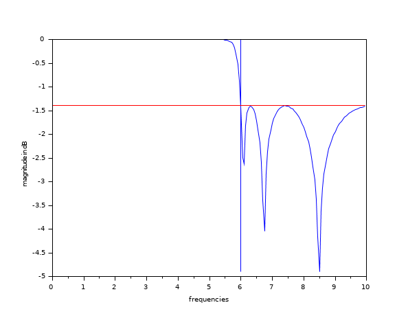
//Chebyshev; ripple in the stopband
n=10;
omegar=6;
A=1/0.2;
Samples=0.0001:0.05:10;
h2=cheb2mag(n,omegar,A,Samples);
plot(Samples,log(h2)/log(10))
xtitle("", "frequencies", "magnitude in dB");

//Plotting of frequency edges
minval=(-max(-log(h2)))/log(10);
plot2d([omegar;omegar],[minval;0],[2],"000");

//Computation of the attenuation in dB at the stopband edge
attenuation=-log(A*A)/log(10);
plot2d(Samples',attenuation*ones(Samples)',[5],"000")
See also
- cheb1mag — response of Chebyshev type 1 filter
| Report an issue | ||
| << cheb1mag | Filters | ell1mag >> |