Rootfinding

Description

Some problems require zero crossing detection of continuous functions (for instance, regulation systems), also named rootfinding. This feature is common to all solvers, and is realized by following the same process.

Each Zero-crossing Block defines one of these functions, noted g(t).

Generally, the feature only finds roots of odd multiplicity, corresponding to changes in sign of g(t). If a user root function has a root of even multiplicity (no sign change), it will probably be missed. If such a root is desired, the user should reformulate the root function so that it changes sign at the desired root.

The basic scheme used is to check for sign changes of any g(t) over each time step taken, and then (when a sign change is found) to home in on the root (or roots) with a modified secant method.

After suitable checking and adjusting has been done, the roots are to be sought within [t_lo, t_hi] . A loop is entered to locate the root to within a rather tight tolerance, given by the unit roudoff, the current time and the step size.

We then determine which root function is more likely to have its roots occur first by comparing the secant method values, and set a new value t_mid and restrain the research interval to either [t_lo, t_mid] or [t_mid, t_hi] , following which does the sign change occur in.

Since the tolerance depends on the step size, the smaller it is, the more accurate the homing in will be.

Examples and Overhead

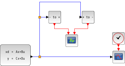
Simple example of a Sine crossing zero several times:

// Import the diagram and set the ending time
loadScicos();
loadXcosLibs();
importXcosDiagram("SCI/modules/xcos/demos/Threshold_ZeroCrossing.zcos");

// Start the timer, launch the simulation and display time
tic();
try xcos_simulate(scs_m, 4); catch disp(lasterror()); end
t = toc();
disp(t, "Time for LSodar:");

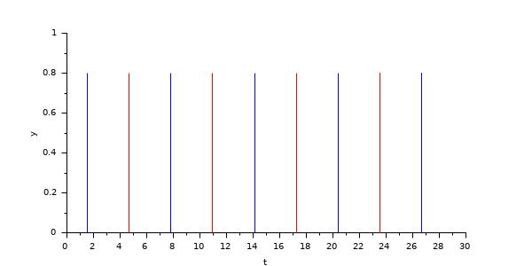
The blue bars represent the "positive to negative" zero crossings, while the red ones are for "negative to positive".

Now, in the two following scripts, we test the computational overhead of the rootfinding with LSodar:

First, a Sine function that crosses zero every π period: Open the script

Time with rootfinding:
 15.021

Time without rootfinding:
 10.573
            

Then, a simple straight line that crosses zero only once, in the middle of the interval: Open the script

Time with rootfinding:
 0.114

Time without rootfinding:
 0.09
            

Following the number of zero crossings, the aspect of the function near these crossings, the tolerances, ..., the computational overhead ranges between 25% and 45%.

See also

• LSodar — LSodar (short for Livermore Solver for Ordinary Differential equations, with Automatic method switching for stiff and nonstiff problems, and with Root-finding) is a numerical solver providing an efficient and stable method to solve Ordinary Differential Equations (ODEs) Initial Value Problems.
• CVode — CVode (short for C-language Variable-coefficients ODE solver) is a numerical solver providing an efficient and stable method to solve Ordinary Differential Equations (ODEs) Initial Value Problems. It uses either BDF or Adams as implicit integration method, and Newton or Functional iterations.
• IDA — Implicit Differential Algebraic equations system solver, providing an efficient and stable method to solve Differential Algebraic Equations system (DAEs) Initial Value Problems.
• Runge-Kutta 4(5) — Runge-Kutta is a numerical solver providing an efficient explicit method to solve Ordinary Differential Equations (ODEs) Initial Value Problems.
• Dormand-Prince 4(5) — Dormand-Prince is a numerical solver providing an efficient explicit method to solve Ordinary Differential Equations (ODEs) Initial Value Problems.
• Implicit Runge-Kutta 4(5) — Numerical solver providing an efficient and stable implicit method to solve Ordinary Differential Equations (ODEs) Initial Value Problems.
• Crank-Nicolson 2(3) — Crank-Nicolson is a numerical solver based on the Runge-Kutta scheme providing an efficient and stable implicit method to solve Ordinary Differential Equations (ODEs) Initial Value Problems. Called by xcos.
• DDaskr — Double-precision Differential Algebraic equations system Solver with Krylov method and Rootfinding: numerical solver providing an efficient and stable method to solve Differential Algebraic Equations systems (DAEs) Initial Value Problems
• Comparisons — This page compares solvers to determine which one is best fitted for the studied problem.
• ode — 常微分方程式ソルバ
• ode_discrete — 常微分方程式ソルバ, 離散時間シミュレーション
• ode_root — 求解付きの常微分方程式ソルバ
• odedc — 離散/連続 ODE ソルバ
• impl — 微分代数方程式

Bibliography

Sundials Documentation