Please note that the recommended version of Scilab is 2026.1.0. This page might be outdated.
However, this page did not exist in the previous stable version.
IDA
Implicit Differential Algebraic equations system solver, providing an efficient and stable method to solve Differential Algebraic Equations system (DAEs) Initial Value Problems.
Description
Called by xcos, IDA (short for Implicit Differential Algebraic equations system solver) is a numerical solver providing an efficient and stable method to solve Initial Value Problems of the form:

Starting then with those y0 and yPrime0 , IDA approximates yn+1 with the BDF formula:

with, like in CVode, yn the approximation of y(tn) , hn = tn - tn-1 the step size, and the coefficients are fixed, uniquely determined by the method type, its order q ranging from 1 to 5 and the history of the step sizes.
Injecting this formula in (1) yields the system:

To apply Newton iterations to it, we rewrite it into:
![J \left[y_{n(m+1)}-y_{n(m)} \right] = -G(y_{n(m)})](/docs/6.0.2/ja_JP/_LaTeX_6-IDA.xml_4.png)
with J an approximation of the Jacobian:

α changes whenever the step size or the method order varies.
An implemented direct dense solver is used and we go on to the next step.
IDA uses the history array to control the local error yn(m) - yn(0) and recomputes hn if that error is not satisfying.
The function is called in between activations, because a discrete activation may change the system.
Following the criticality of the event (its effect on the continuous problem), we either relaunch the solver with different start and final times as if nothing happened, or, if the system has been modified, we need to "cold-restart" the problem by reinitializing it anew and relaunching the solver.
Averagely, IDA accepts tolerances up to 10-11. Beyond that, it returns a Too much accuracy requested error.
Example
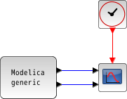
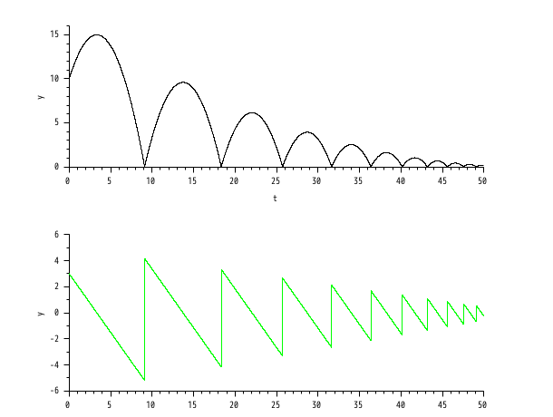
The 'Modelica Generic' block returns its continuous states, we can evaluate them with IDA by running the example:
See also
- LSodar — LSodar (short for Livermore Solver for Ordinary Differential equations, with Automatic method switching for stiff and nonstiff problems, and with Root-finding) is a numerical solver providing an efficient and stable method to solve Ordinary Differential Equations (ODEs) Initial Value Problems.
- CVode — CVode (short for C-language Variable-coefficients ODE solver) is a numerical solver providing an efficient and stable method to solve Ordinary Differential Equations (ODEs) Initial Value Problems. It uses either BDF or Adams as implicit integration method, and Newton or Functional iterations.
- Runge-Kutta 4(5) — Runge-Kutta is a numerical solver providing an efficient explicit method to solve Ordinary Differential Equations (ODEs) Initial Value Problems.
- Dormand-Prince 4(5) — Dormand-Prince is a numerical solver providing an efficient explicit method to solve Ordinary Differential Equations (ODEs) Initial Value Problems.
- Implicit Runge-Kutta 4(5) — Numerical solver providing an efficient and stable implicit method to solve Ordinary Differential Equations (ODEs) Initial Value Problems.
- Crank-Nicolson 2(3) — Crank-Nicolson is a numerical solver based on the Runge-Kutta scheme providing an efficient and stable implicit method to solve Ordinary Differential Equations (ODEs) Initial Value Problems. Called by xcos.
- DDaskr — Double-precision Differential Algebraic equations system Solver with Krylov method and Rootfinding: numerical solver providing an efficient and stable method to solve Differential Algebraic Equations systems (DAEs) Initial Value Problems
- Comparisons — This page compares solvers to determine which one is best fitted for the studied problem.
- ode — 常微分方程式ソルバ
- ode_discrete — 常微分方程式ソルバ, 離散時間シミュレーション
- ode_root — 求解付きの常微分方程式ソルバ
- odedc — 離散/連続 ODE ソルバ
- impl — 微分代数方程式
Bibliography
| Report an issue | ||
| << Crank-Nicolson 2(3) | Solvers | DDaskr >> |