Please note that the recommended version of Scilab is 2026.1.0. This page might be outdated.
See the recommended documentation of this function
Dormand-Prince 4(5)
Dormand-Prince is a numerical solver providing an efficient explicit method to solve Ordinary Differential Equations (ODEs) Initial Value Problems.
Description
Called by xcos, Dormand-Prince is a numerical solver providing an efficient fixed-size step method to solve Initial Value Problems of the form:

CVode and IDA use variable-size steps for the integration.
A drawback of that is the unpredictable computation time. With Dormand-Prince, we do not adapt to the complexity of the problem, but we guarantee a stable computation time.
As of now, this method is explicit, so it is not concerned with Newton or Functional iterations, and not advised for stiff problems.
It is an enhancement of the Euler method, which approximates yn+1 by truncating the Taylor expansion.
By convention, to use fixed-size steps, the program first computes a fitting h that approaches the simulation parameter max step size.
An important difference of Dormand-Prince with the previous methods is that it computes up to the seventh derivative of y, while the others only use linear combinations of y and y'.
Here, the next value is determined by the present value yn plus the weighted average of six increments, where each increment is the product of the size of the interval, h, and an estimated slope specified by the function f(t,y):
- k1 is the increment based on the slope at the beginning of the interval, using yn (Euler's method),
- k2, k3, k4 and k5 are the increments based on the slope at respectively 0.2, 0.3, 0.8 and 0.9 of the interval, using combinations of each other,
- k6 is the increment based on the slope at the end, also using combinations of the other ki.
We can see that with the ki, we progress in the derivatives of yn . In the computation of the ki, we deliberately use coefficients that yield an error in O(h5) at every step.
So the total error is number of steps * O(h5) . And since number of steps = interval size / h by definition, the total error is in O(h4) .
That error analysis baptized the method Dormand-Prince 4(5): O(h5) per step, O(h4) in total.
Althought the solver works fine for max step size up to 10-3 , rounding errors sometimes come into play as it approaches 4*10-4 . Indeed, the interval splitting cannot be done properly and we get capricious results.
Examples
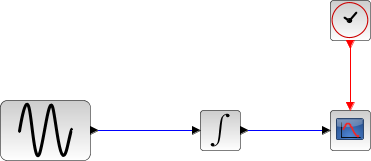
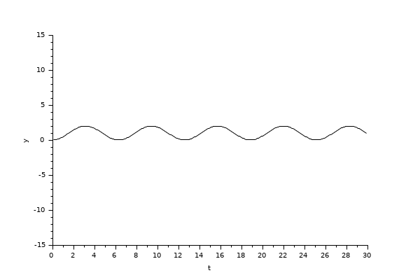
The integral block returns its continuous state, we can evaluate it with Dormand-Prince by running the example:
// Import the diagram and set the ending time
loadScicos();
loadXcosLibs();
importXcosDiagram("SCI/modules/xcos/examples/solvers/ODE_Example.zcos");
scs_m.props.tf = 5000;

// Select the Dormand-Prince solver and set the precision
scs_m.props.tol(6) = 5;
scs_m.props.tol(7) = 10^-2;

// Start the timer, launch the simulation and display time
tic();
try xcos_simulate(scs_m, 4); catch disp(lasterror()); end
t = toc();
disp(t, "Time for Dormand-Prince:");
The Scilab console displays:
Time for Dormand-Prince:
 9.197
Now, in the following script, we compare the time difference between Dormand-Prince and CVode by running the example with the five solvers in turn: Open the script
Time for BDF / Newton:
 18.894

Time for BDF / Functional:
 18.382

Time for Adams / Newton:
 10.368

Time for Adams / Functional:
 9.815

Time for Dormand-Prince:
 7.842
These results show that on a nonstiff problem, for relatively same precision required and forcing the same step size, Dormand-Prince's computational overhead (compared to Runge-Kutta) is significant and is close to Adams/Functional. Its error to the solution is althought much smaller than the regular Runge-Kutta 4(5), for a small overhead in time.
Variable-size step ODE solvers are not appropriate for deterministic real-time applications because the computational overhead of taking a time step varies over the course of an application.
See also
- LSodar — LSodar (short for Livermore Solver for Ordinary Differential equations, with Automatic method switching for stiff and nonstiff problems, and with Root-finding) is a numerical solver providing an efficient and stable method to solve Ordinary Differential Equations (ODEs) Initial Value Problems.
- CVode — CVode (short for C-language Variable-coefficients ODE solver) is a numerical solver providing an efficient and stable method to solve Ordinary Differential Equations (ODEs) Initial Value Problems. It uses either BDF or Adams as implicit integration method, and Newton or Functional iterations.
- IDA — Implicit Differential Algebraic equations system solver, providing an efficient and stable method to solve Differential Algebraic Equations system (DAEs) Initial Value Problems.
- Runge-Kutta 4(5) — Runge-Kutta is a numerical solver providing an efficient explicit method to solve Ordinary Differential Equations (ODEs) Initial Value Problems.
- Implicit Runge-Kutta 4(5) — Numerical solver providing an efficient and stable implicit method to solve Ordinary Differential Equations (ODEs) Initial Value Problems.
- Crank-Nicolson 2(3) — Crank-Nicolson is a numerical solver based on the Runge-Kutta scheme providing an efficient and stable implicit method to solve Ordinary Differential Equations (ODEs) Initial Value Problems. Called by xcos.
- DDaskr — Double-precision Differential Algebraic equations system Solver with Krylov method and Rootfinding: numerical solver providing an efficient and stable method to solve Differential Algebraic Equations systems (DAEs) Initial Value Problems
- Comparisons — This page compares solvers to determine which one is best fitted for the studied problem.
- ode — 常微分方程式ソルバ
- ode_discrete — 常微分方程式ソルバ, 離散時間シミュレーション
- ode_root — 求解付きの常微分方程式ソルバ
- odedc — 離散/連続 ODE ソルバ
- impl — 微分代数方程式
Bibliography
Journal of Computational and Applied Mathematics, Volume 15, Issue 2, 2 June 1986, Pages 203-211 Dormand-Prince Method
History
| バージョン | 記述 |
| 5.4.1 | Dormand-Prince 4(5) solver added |
| Report an issue | ||
| << Runge-Kutta 4(5) | Solvers | Implicit Runge-Kutta 4(5) >> |