Please note that the recommended version of Scilab is 2026.1.0. This page might be outdated.
See the recommended documentation of this function
Comparisons
This page compares solvers to determine which one is best fitted for the studied problem.
Introduction
Following the type of problem, finding out which method to use is not always obvious, only general guidelines can be established. Those are discussed in this page.
Variable-size and Fixed-size
The solvers can be divided into two distinct main families: the Variable-size and the Fixed-size step methods.
They both compute the next simulation time as the sum of the current simulation time and a quantity known as the step size, which is constant in the Fixed-size solvers and can change in the Variable-size ones, depending on the model dynamics and the input tolerances.
If looking for stable computation time, the user should select a Fixed-size step solver, because the computation overhead for a Variable-size step method cannot be properly predicted.
Although for a simple problem (or loose tolerances) a Variable-size solver can significantly improve the simulation time by computing bigger step sizes, a Fixed-size method is preferable if the ideal step size is known and roughly constant (the user should then mention it in max step size).
Variable-size step solvers:
- LSodar
- CVode
- IDA
- Runge-Kutta 4(5)
- Dormand-Prince 4(5)
- Implicit Runge-Kutta 4(5)
- Crank-Nicolson 2(3)
Variable step-size ODE solvers are not appropriate for deterministic real-time applications because the computational overhead of taking a time step varies over the course of an application.
Explicit and Implicit - Stiffness
Within these two families, we can distinguish Explicit solvers from Implicit ones.
While explicit methods only use data available on the current step, the implicit ones will attempt to compute derivatives at further times. In order to do this, they use nonlinear solvers such as fixed-point iterations, functional iterations (nonstiff) or modified Newton methods (stiff).
The family choice is usually determined by the stiffness of the problem, which is, when there is a big gap between the biggest and the smallest eigen values modules of the jacobian matrix (when it is ill-conditionned). It is generally a system that is sensitive to discontinuitues, meaning that the required precision is not constant.
Implicit solvers:
- LSodar
- CVode
- IDA
- Implicit Runge-Kutta 4(5)
- Crank-Nicolson 2(3)
- Runge-Kutta 4(5)
- Dormand-Prince 4(5)
To put it simply, the Explicit go straight to a computation of the solution, whereas the Implicit concentrate on stability, involving more operations, following the tolerances.
So how to choose?
Because it is not possible to know for sure whether a solver will be efficient for a given system or not, the best way is to run the most probable one on it and to compare their results.
The user should first establish the complexity of his problem (stability / stiffness) and if he desires high precision, rapid simulation, predictable time or an automated program.
Precision: CVode,
Predictable time: Fixed-size step,
Simulation time: LSodar,
Automated: LSodar.
Examples - ODEs
We will begin with a simple nonstiff example: a Sine integration.
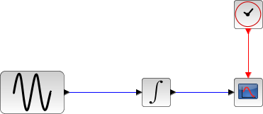
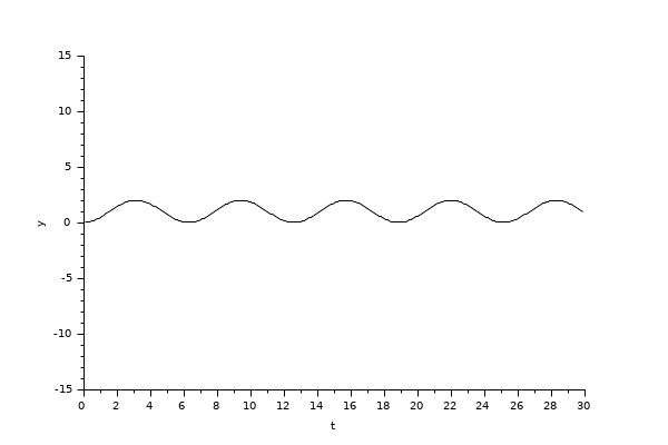
In the following script, we compare the time difference between the solvers by running the example with the nine solvers in turn (IDA doesn't handle this kind of problem): Open the script
The Scilab console displays:
Time for LSodar:
 10.1

Time for CVode BDF/Newton:
 31

Time for CVode BDF/Functional:
 30

Time for CVode Adams/Newton:
 17.211

Time for CVode Adams/Functional:
 16.305

Time for Dormand-Prince:
 12.92

Time for Runge-Kutta:
 7.663

Time for implicit Runge-Kutta:
 10.881

Time for Crank-Nicolson:
 7.856
These results show that on a nonstiff problem and for same precision required, Runge-Kutta is fastest.
In spite of the computational overhead of the step size, LSodar is not too distant from the Fixed-size solvers because it is able to take long steps.
From the results, we can extract speed factors and set the following table:
| BDF / Newton | BDF / Functional | Adams / Newton | Adams / Functional | Dormand-Prince | Runge-Kutta | Implicit Runge-Kutta | Crank-Nicolson | |
| LSodar | 3.1x | 3x | 1.7x | 1.6x | 1.3x | 0.75x | 1.08x | .07x |
| BDF / Newton | 0.1x | 0.6x | 0.5x | 0.4x | 0.25x | 0.35x | 0.23x | |
| BDF / Functional | 0.6x | 0.5x | 0.4x | 0.25x | 0.4x | 0.24x | ||
| Adams / Newton | 0.9x | 0.75x | 0.45x | 0.6x | 0.42x | |||
| Adams / Functional | 0.8x | 0.5x | 0.7x | 0.45x | ||||
| Dormand-Prince | 0.6x | 0.8x | 0.56x | |||||
| Runge-Kutta | 1.4x | 0.95x | ||||||
| Implicit Runge-Kutta | 0.67x |
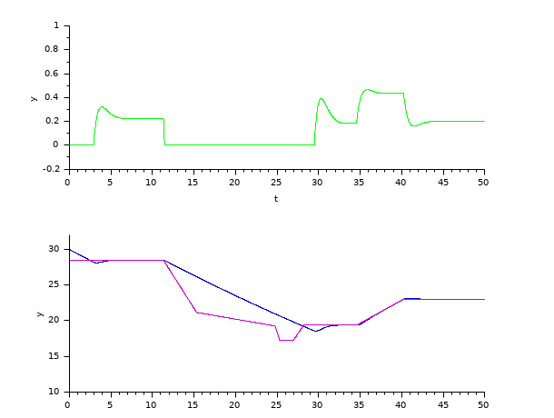
Next, a basic controller with six continuous states is tested.
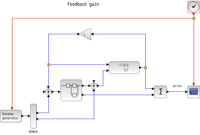

In the following script, we compare the time difference between the solvers by running the example with the nine solvers in turn (IDA doesn't handle this kind of problem): Open the script
The Scilab console displays:
Time for LSodar:
 10

Time for CVode BDF/Newton:
 28.254

Time for CVode BDF/Functional:
 25.545

Time for CVode Adams/Newton:
 15

Time for CVode Adams/Functional:
 12.1

Time for Dormand-Prince:
 2.359

Time for Runge-Kutta:
 1.671

Time for implicit Runge-Kutta:
 5.612

Time for Crank-Nicolson:
 3.345
These results show that as stiffness appears, BDF / Newton starts picking up speed. But the problem is not yet complicated enough for that method to be interesting.
The updated speed factors table is as follows:
| BDF / Newton | BDF / Functional | Adams / Newton | Adams / Functional | Dormand-Prince | Runge-Kutta | Implicit Runge-Kutta | Crank-Nicolson | |
| LSodar | 2.8x | 2.6x | 1.5x | 1.2x | 0.2x | 0.17x | 0.5x | 0.33x |
| BDF / Newton | 0.9x | 0.5x | 0.4x | 0.1x | 0.05x | 0.2x | 0.12x | |
| BDF / Functional | 0.6x | 0.5x | 0.1x | 0.07x | 0.2x | 0.13x | ||
| Adams / Newton | 0.8x | 0.15x | 0.1x | 0.4x | 0.22x | |||
| Adams / Functional | 0.2x | 0.1x | 0.5x | 0.28x | ||||
| Dormand-Prince | 0.7x | 2.4x | 1.42x | |||||
| Runge-Kutta | 3.4x | 2x | ||||||
| Implicit Runge-Kutta | 0.6x |
Now, we use Kalman's filter, which contains fifteen continuous states.
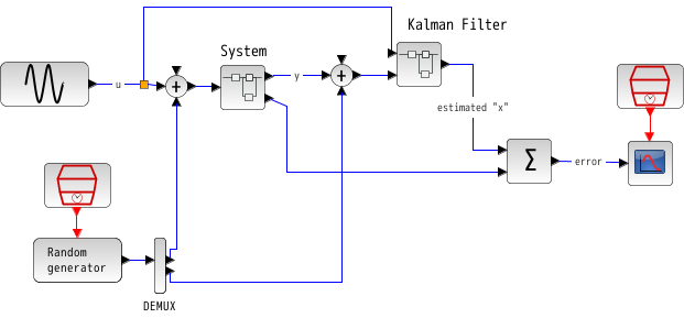
In the following script, we compare the time difference between the solvers by running the example with the nine solvers in turn (IDA doesn't handle this kind of problem): Open the script
The Scilab console displays:
Time for LSodar:
 10

Time for CVode BDF/Newton:
 21.3

Time for CVode BDF/Functional:
 15.8

Time for CVode Adams/Newton:
 12.5

Time for CVode Adams/Functional:
 8.67

Time for Dormand-Prince:
 1.244

Time for Runge-Kutta:
 0.87

Time for implicit Runge-Kutta:
 4

Time for Crank-Nicolson:
 2.657
These results show that for a bigger problem (more continuous states implies more equations), the Newton iteration starts showing interest, for it comes closer to the other solvers.
The updated speed factors table is as follows:
| BDF / Newton | BDF / Functional | Adams / Newton | Adams / Functional | Dormand-Prince | Runge-Kutta | Implicit Runge-Kutta | Crank-Nicolson | |
| LSodar | 2.1x | 1.6x | 1.3x | 0.85x | 0.1x | 0.1x | 0.4x | 0.26x |
| BDF / Newton | 0.75x | 0.6x | 0.4x | 0.06x | 0.05x | 0.2x | 0.12x | |
| BDF / Functional | 0.8x | 0.55x | 0.08x | 0.06x | 0.25x | 0.17x | ||
| Adams / Newton | 0.7x | 0.1x | 0.07x | 0.3x | 0.21x | |||
| Adams / Functional | 0.15x | 0.1x | 0.5x | 0.3x | ||||
| Dormand-Prince | 0.7x | 3.2x | 2.1x | |||||
| Runge-Kutta | 4.6x | 3.1x | ||||||
| Implicit Runge-Kutta | 0.66x |
Examples - DAEs
In this section we compare IDA with DDaskr.
Example: a bouncing ball.
In the following script, we compare the time difference between the solvers by running the example with the three solvers in turn: Open the script
The Scilab console displays:
Time for IDA:
 8

Time for DDaskr - Newton:
 5.6

Time for DDaskr - GMRes:
 6.5
This result shows that on a stiff problem, with rootfinding and for same precision required, DDaskr - Newton is fastest.
The difference in time is attributed to the powerful implementation of DDaskr and its least error control.
GMRes is slower due to the small size of the problem.
From the results, we can extract the speed factors:
| IDA | DDaskr G | |
| DDaskr N | 1.39x | 1.9x |
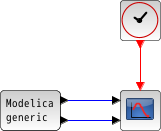
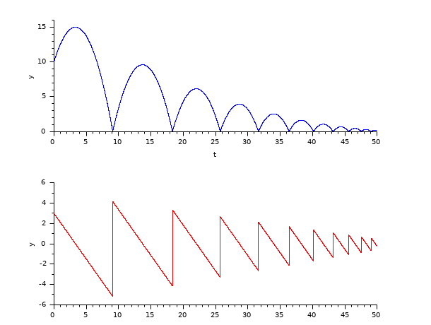
The next example simply corroborates the previous one, it is shorter but more thorough, since it deals with the filling and emptying of a tank.
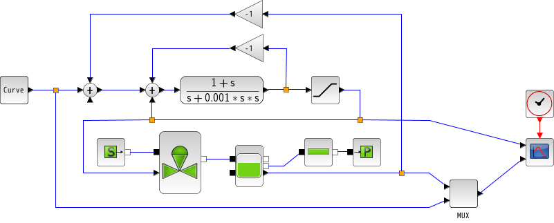
In the following script, we compare the time difference between the solvers by running the example with the three solvers in turn: Open the script
The Scilab console displays:
Time for IDA:
 3

Time for DDaskr - Newton:
 0.8

Time for DDaskr - GMRes:
 0.85
From the results, we can extract the speed factors:
| IDA | DDaskr G | |
| DDaskr N | 3.75x | 1.06x |
See also
- LSodar — LSodar (short for Livermore Solver for Ordinary Differential equations, with Automatic method switching for stiff and nonstiff problems, and with Root-finding) is a numerical solver providing an efficient and stable method to solve Ordinary Differential Equations (ODEs) Initial Value Problems.
- CVode — CVode (short for C-language Variable-coefficients ODE solver) is a numerical solver providing an efficient and stable method to solve Ordinary Differential Equations (ODEs) Initial Value Problems. It uses either BDF or Adams as implicit integration method, and Newton or Functional iterations.
- IDA — Implicit Differential Algebraic equations system solver, providing an efficient and stable method to solve Differential Algebraic Equations system (DAEs) Initial Value Problems.
- Runge-Kutta 4(5) — Runge-Kutta is a numerical solver providing an efficient explicit method to solve Ordinary Differential Equations (ODEs) Initial Value Problems.
- Dormand-Prince 4(5) — Dormand-Prince is a numerical solver providing an efficient explicit method to solve Ordinary Differential Equations (ODEs) Initial Value Problems.
- Implicit Runge-Kutta 4(5) — Numerical solver providing an efficient and stable implicit method to solve Ordinary Differential Equations (ODEs) Initial Value Problems.
- Crank-Nicolson 2(3) — Crank-Nicolson is a numerical solver based on the Runge-Kutta scheme providing an efficient and stable implicit method to solve Ordinary Differential Equations (ODEs) Initial Value Problems. Called by xcos.
- DDaskr — Double-precision Differential Algebraic equations system Solver with Krylov method and Rootfinding: numerical solver providing an efficient and stable method to solve Differential Algebraic Equations systems (DAEs) Initial Value Problems
- ode — 常微分方程式ソルバ
- ode_discrete — 常微分方程式ソルバ, 離散時間シミュレーション
- ode_root — 求解付きの常微分方程式ソルバ
- odedc — 離散/連続 ODE ソルバ
- impl — 微分代数方程式
| Report an issue | ||
| << Rootfinding | Solvers | xcos >> |