Please note that the recommended version of Scilab is 2026.1.0. This page might be outdated.
See the recommended documentation of this function
lqg
LQG compensator
Syntax
K=lqg(P_aug,r)
K=lqg(P,Qxu,Qwv)
K=lqg(P,Qxu,Qwv,Qi,#dof)
Arguments
- P_aug
State space representation of the augmented plant (see: lqg2stan)
- r
1 by 2 row vector = (number of measurements, number of inputs) (dimension of the 2,2 part of
P_aug)- P
State-space representation of the nominal plant (
nuinputs,nyoutputs,nxstates).- Qxu
Symmetric
nx+nubynx+nuweighting matrix.- Qwv
Symmetric
nx+nybynx+nycovariance matrix.- Qi
Symmetric
nybynyweight for integral term.- #dof
Scalar with value in {1,2}, the degrees of freedom of the controller. The default value is 2.
- K
Linear LQG (H2) controller in state-space representation.
Description
Regulation around zero
- Syntax
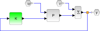
K=lqg(P_aug,r)Computes the linear optimal LQG (H2) controller for the "augmented" plant
P_augwhich can be generated by lqg2stan givent the nominal plant plantP, the weighting matrixQxuand the noise covariance matrixQwv. - Syntax
K=lqg(P,Qxu,Qwv)Computes the linear optimal LQG (H2) controller for the nominal plant
P, the weighting matrixQxuand the noise covariance matrixQwv
Regulation around a reference signal, Syntax K=lqg(P,Qxu,Qwv,Qi [,#dof])
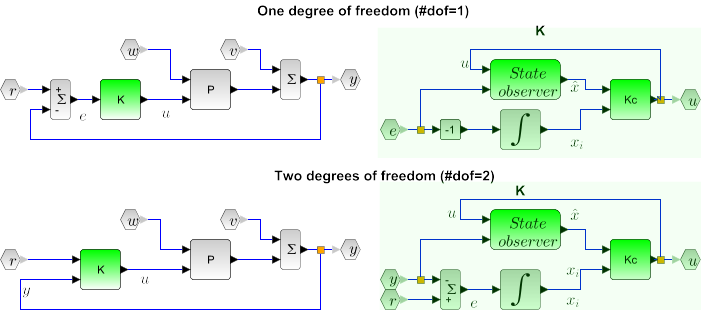
Computes the linear optimal LQG (H2) reference tracking controller for the
plant P, the weighting matrix
Qxu and the noise covariance matrix
Qwv
Examples
Assume the dynamical system formed by two masses connected by a spring and a damper:
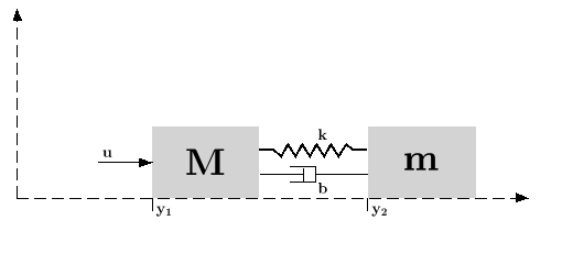
A force  (where
  is a
noise) is applied to M, the deviations
is a
noise) is applied to M, the deviations  and
and
 from equilibrium positions of the masses are
measured. These measures are subject to an additionnal
noise
from equilibrium positions of the masses are
measured. These measures are subject to an additionnal
noise  .
.
A continuous time state space representation of this system is:


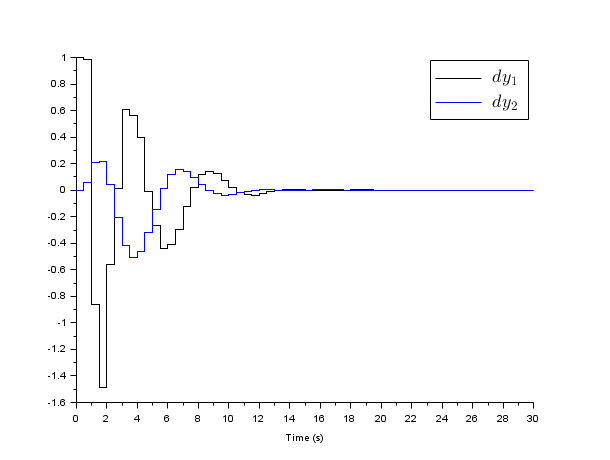
The instructions below can be used to compute a LQG compensator
of the discretized version of this dynamical
system.  and
and  are discrete
time white noises such as
are discrete
time white noises such as

The LQ cost is defined by

Regulation around zero
// Form the state space model
M = 1; m = 0.2; k = 0.1; b = 0.004;
A = [0     1    0    0
-k/M  -b/M  k/M  b/M
0     0    0    1
k/m  b/m  -k/m  -b/m];
B = [0; 1/M; 0; 0];
C = [1 0 0 0  //dy1
0 0 1 0];//dy2
//inputs u and e; outputs dy1 and dy2
P = syslin("c",A, B, C);
// Discretize it
dt=0.5;
Pd=dscr(P, dt);

// The noise variances
Q_e=1; //additive input noise variance
R_vv=0.0001*eye(2,2); //measurement noise variance
Q_ww=Pd.B*Q_e*Pd.B'; //input noise adds to regular input u
Qwv=sysdiag(Q_ww,R_vv);
//The compensator weights
Q_xx=diag([0.1 0 5 0]); //Weights on states
R_uu   = 0.3; //Weight on input
Qxu=sysdiag(Q_xx,R_uu);

//----syntax [K,X]=lqg(P,Qxu,Qwv)---
J=lqg(Pd,Qxu,Qwv);

//----syntax [K,X]=lqg(P_aug,r)---
// Form standard LQG model
[Paug,r]=lqg2stan(Pd,Qxu,Qwv); // Form standard LQG model
J1=lqg(Paug,r);

//  Form the closed loop
Sys=Pd/.(-J);
// Compare real and Estimated states for initial state evolution
t = 0:dt:30;
// Simulate system evolution for initial state [1;0;0;0;
y = flts(zeros(t),Sys,eye(8,1));
clf;
plot2d(t',y')
e=gce();e.children.polyline_style=2;
L=legend(["$dy_1$","$dy_2$"]);L.font_size=4;
xlabel('Time (s)')
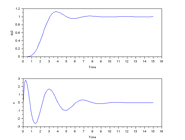
Regulation around a reference signal, Syntax K=lqg(P,Qxu,Qwv,Qi [,#dof])
The purpose of the controller is here to assign
 using the measure of
  .
.
M = 1; m = 0.2; k = 0.1; b = 0.004;
A = [0     1    0    0
-k/M  -b/M  k/M  b/M
0     0    0    1
k/m  b/m  -k/m  -b/m];
B = [0; 1/M; 0; 0];
C = [1 0 0 0  //dy1
0 0 1 0];//dy2
//inputs u and e; outputs dy1 and dy2
P = syslin("c",A, B, C);
// Discretize it
dt=0.1;
Pd=dscr(P, dt);

// The noise variances
Q_e=1; //additive input noise variance
R_vv=0.0001; //measurement noise variance
Q_ww=Pd.B*Q_e*Pd.B'; //input noise adds to regular input u
Qwv=sysdiag(Q_ww,R_vv);
//The compensator weights
Q_xx=diag([0.1 0 1 0]); //Weights on states
R_uu   = 0.1; //Weight on input
Qxu=sysdiag(Q_xx,R_uu);

//Control of the second mass position (y2)
Qi=50;
J=lqg(Pd(2,:),Qxu,Qwv,Qi);
H=lft([1;1]*Pd(2,:)*(-J),1);
//step response
t=0:dt:15;
r=ones(t);
dy2=flts(r,H);
clf;
subplot(211);plot(t',dy2');xlabel("Time");ylabel("dy2")
u=flts([r;dy2],J);
subplot(212);plot(t',u');xlabel("Time");ylabel("u")
Reference
Engineering and Scientific Computing with Scilab, Claude Gomez and al.,Springer Science+Business Media, LLC,1999, ISNB:978-1-4612-7204-5
See Also
| Report an issue | ||
| << lqe | Linear Quadratic | lqg2stan >> |