Please note that the recommended version of Scilab is 2026.1.0. This page might be outdated.
See the recommended documentation of this function
lqr
LQ compensator (full state)
Syntax
[K,X]=lqr(P12)
[K,X]=lqr(P,Q,R [,S])
Arguments
- P12
A state space representation of a linear dynamical system (see syslin)
- P
A state space representation of a linear dynamical system (see syslin)
- Q
Real symmetric matrix, with same dimensions as P.A
- R
full rank real symmetric matrix
- S
real matrix, the default value is
zeros(size(R,1),size(Q,2))- K
a real matrix, the optimal gain
- X
a real symmetric matrix, the stabilizing solution of the Riccati equation
Description
- Syntax
[K,X]=lqr(P) Computes the linear optimal LQ full-state gain K for the state space representation P
And instantaneous cost function in l2-norm:

- Syntax
[K,X]=lqr(P,Q,R [,S]) Computes the linear optimal LQ full-state gain K for the linear dynamical system P:
And instantaneous cost function in l2-norm:


Remark
In this case the P.C and P.D componants of the system are ignored
Algorithm
For a continuous plant, if
 is the stabilizing solution of the Riccati equation:
the linear optimal LQ full-state gain K is given by
is the stabilizing solution of the Riccati equation:
the linear optimal LQ full-state gain K is given by

For a discrete plant, if
 is the stabilizing solution of the Riccati equation:
the linear optimal LQ full-state gain K is given by
is the stabilizing solution of the Riccati equation:
the linear optimal LQ full-state gain K is given by

An equivalent form for the equation is
with

The gain K is such that  is stable.
The resolution of the Riccati equation is obtained by schur factorization of the 3-blocks matrix pencils associated with these Riccati equations:
For a continuous plant

For a discrete time plant

Caution
It is assumed that matrix  or
or  is non singular.
Remark
If the full state of the system is not available, An estimator can be built using the lqe or the lqg function.
Examples
Assume the dynamical system formed by two masses connected by a spring and a damper:
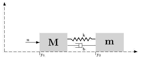
 (where
  is a noise) is applied to the big one. Here it is assumed
that the deviations from equilibrium positions of the mass
is a noise) is applied to the big one. Here it is assumed
that the deviations from equilibrium positions of the mass
 and
and  positions has
well as their derivatives are measured.
positions has
well as their derivatives are measured.
A state space representation of this system is:


The LQ cost is defined by

The following instructions may be used to compute a LQ compensator of this dynamical system.
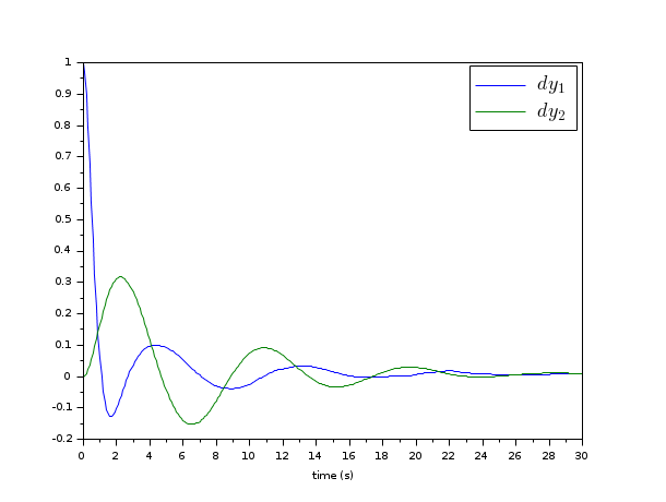
// Form the state space model (assume full state output)
M = 1; m = 0.2; k = 0.1; b = 0.004;
A = [  0     1    0    0
-k/M  -b/M  k/M  b/M
0     0    0    1
k/m  b/m  -k/m  -b/m];
B = [0; 1/M; 0; 0];
C = eye(4,4);
P = syslin("c",A, B, C);
//The compensator weights
Q_xx=diag([15 0 3 0]); //Weights on states
R_uu   = 0.5; //Weight on input
Kc=lqr(P,Q_xx,R_uu);

//form the Plant+compensator system

C=[1 0 0 0  //dy1
0 0 1 0];//dy2
S=C*(P/.(-Kc));
//check system stability
and(real(spec(S.A))<0)
// Check by simulation
dt=0.1;
t=0:dt:30;
u=0.1*rand(t);
y=csim(u,t,S,[1;0;0;0]);
clf;plot(t',y');xlabel(_("time (s)"))
L=legend(["$dy_1$","$dy_2$"]);L.font_size=4;
Reference
Engineering and Scientific Computing with Scilab, Claude Gomez and al.,Springer Science+Business Media, LLC,1999, ISNB:978-1-4612-7204-5
See also
| Report an issue | ||
| << lqi | Linéaire Quadratique | Placement de pôles >> |