Please note that the recommended version of Scilab is 2026.1.0. This page might be outdated.
See the recommended documentation of this function
lqe
linear quadratic estimator (Kalman Filter)
Syntax
[K,X]=lqe(Pw)
[K,X]=lqe(P,Qww,Rvv [,Swv])
Arguments
- Pw
A state space representation of a linear dynamical system (see syslin)
- P
A state space representation of a linear dynamical system (
nuinputs,nyoutputs,nxstates) (see syslin)- Qww
Real
nxbynxsymmetric matrix, the process noise variance- Rvv
full rank real
nybynysymmetric matrix, the measurement noise variance.- Swv
real
nxbynymatrix, the process noise vs measurement noise covariance. The default value is zeros(nx,ny).- K
a real matrix, the optimal gain.
- X
a real symmetric matrix, the stabilizing solution of the Riccati equation.
Description
This function computes the linear optimal LQ estimator gain of the state estimator for a detectable (see dt_ility) linear dynamical system and the variance matrices for the process and the measurement noises.
Syntax [K,X]=lqe(P,Qww,Rvv [,Swv])
Computes the linear optimal LQ estimator gain K for the dynamical system:


Where  are white noises such
as
are white noises such
as 
 | CautionThe values of |


| Standard form     is now a white noise such
as is now a white noise such
as  |
Syntax [K,X]=lqe(Pw)
Computes the linear optimal LQ estimator gain K for the dynamical system

Where  is a white noise with unit covariance.
Properties
 is stable.
the state estimator is given by the dynamical system:

or
It minimizes the covariance of the steady state error
 .
.For discrete time systems the state estimator is such that:
 (one-step predicted
  ).
).
Algorithm
let  ,
,  and
and 
For the continuous time case K is given by

where
Xis the solution of the stabilizing Riccati equation
For the discrete time case K is given by

where
Xis the solution of the stabilizing Riccati equation
Examples
Assume the dynamical system formed by two masses connected by a spring and a damper:
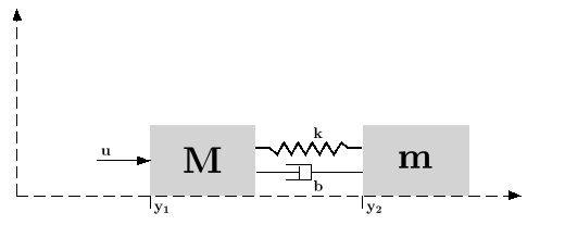
 (where
  is a noise) is applied to the big one, the deviations from equilibrium positions
  and
and  of the masses are measured. These measures are also subject to an additionnal noise
  .
.
A continuous time state space representation of this system is:


 and
and  are discrete time white noises such as

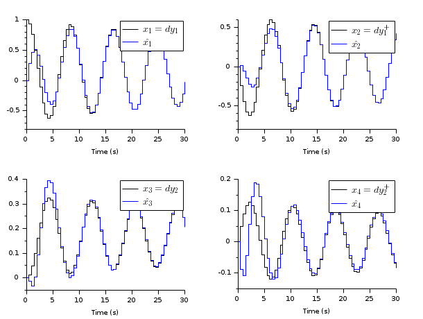
The instructions below can be used to compute a LQ state observer of the discretized version of this dynamical system.
// Form the state space model
M = 1; m = 0.2; k = 0.1; b = 0.004;
A = [  0     1    0    0
      -k/M  -b/M  k/M  b/M
       0     0    0    1
      k/m  b/m  -k/m  -b/m];
B = [0; 1/M; 0; 0];
C = [1 0 0 0  //dy1
     0 0 1 0];//dy2
//inputs u and e; outputs dy1 and dy2
P = syslin("c",A, B, C);
// Discretize it
dt=0.5;
Pd=dscr(P, dt);

//  Set the noise covariance matrices
Q_e=0.01; //additive input noise variance
R_vv=0.001*eye(2,2); //measurement noise variance
Q_ww=Pd.B*Q_e*Pd.B'; //input noise adds to regular input u

//----syntax [K,X]=lqe(P,Qww,Rvv [,Swv])---
Ko=lqe(Pd,Q_ww,R_vv); //observer gain

//----syntax [K,X]=lqe(P21)---
bigR =sysdiag(Q_ww, R_vv);
[W,Wt]=fullrf(bigR);
Bw=W(1:size(Pd.B,1),:);
Dw=W(($+1-size(Pd.C,1)):$,:);
Pw=syslin(Pd.dt,Pd.A,Bw,Pd.C,Dw);
Ko1=lqe(Pw); //same observer gain

//Check gains equality
norm(Ko-Ko1,1)

// Form the observer
O=observer(Pd,Ko);
//check stability
and(abs(spec(O.A))<1)
// Check by simulation
// Modify Pd to make it return the state
Pdx=Pd;Pdx.C=eye(4,4);Pdx.D=zeros(4,1);
t=0:dt:30;
u=zeros(t);
x=flts(u,Pdx,[1;0;0;0]);//state evolution
y=Pd.C*x;
// simulate the observer
x_hat=flts([u+0.01*rand(u);y+0.0001*rand(y)],O);
clf;
subplot(2,2,1)
  plot2d(t',[x(1,:);x_hat(1,:)]'),
  e=gce();e.children.polyline_style=2;
  L=legend('$x_1=dy_1$', '$\hat{x_1}$');L.font_size=3;
  xlabel('Time (s)')
subplot(2,2,2)
  plot2d(t',[x(2,:);x_hat(2,:)]')
  e=gce();e.children.polyline_style=2;
  L=legend('$x_2=dy_1^+$', '$\hat{x_2}$');L.font_size=3;
  xlabel('Time (s)')
subplot(2,2,3)
  plot2d(t',[x(3,:);x_hat(3,:)]')
  e=gce();e.children.polyline_style=2;
  L=legend('$x_3=dy_2$', '$\hat{x_3}$');L.font_size=3;
  xlabel('Time (s)')
subplot(2,2,4)
  plot2d(t',[x(4,:);x_hat(4,:)]')
  e=gce();e.children.polyline_style=2;
  L=legend('$x_4=dy_2^+$', '$\hat{x_4}$');L.font_size=3;
  xlabel('Time (s)')
Reference
Engineering and Scientific Computing with Scilab, Claude Gomez and al.,Springer Science+Business Media, LLC,1999, ISNB:978-1-4612-7204-5
See also
| Report an issue | ||
| << leqr | Linéaire Quadratique | lqg >> |