Please note that the recommended version of Scilab is 2026.1.0. This page might be outdated.
See the recommended documentation of this function
splin2d
bicubic spline gridded 2d interpolation
Calling Sequence
C = splin2d(x, y, z, [,spline_type])
Arguments
- x
a 1-by-nx matrix of doubles, the x coordinate of the interpolation points. We must have x(i)<x(i+1), for i=1,2,...,nx-1.
- y
a 1-by-ny matrix of doubles, the y coordinate of the interpolation points. We must have y(i)<y(i+1), for i=1,2,...,ny-1.
- z
a nx-by-ny matrix of doubles, the function values.
- spline_type
a 1-by-1 matrix of strings, the typof of spline to compute. Available values are spline_type="not_a_knot" and spline_type="periodic".
- C
the coefficients of the bicubic patches. This output argument of splin2d is the input argument of the interp2d function.
Description
This function computes a bicubic spline or sub-spline
s which interpolates the
(xi,yj,zij) points, ie, we have
s(xi,yj)=zij for all i=1,..,nx
and j=1,..,ny. The resulting spline
s is defined by the triplet
(x,y,C) where C is the vector (of
length 16(nx-1)(ny-1)) with the coefficients of each of the (nx-1)(ny-1)
bicubic patches : on [x(i) x(i+1)]x[y(j) y(j+1)],
s is defined by :

The evaluation of s at some points must be done
by the interp2d function. Several kind of
splines may be computed by selecting the appropriate
spline_type parameter. The method used to compute the
bicubic spline (or sub-spline) is the old fashionned one 's, i.e. to
compute on each grid point (xi,yj) an approximation
of the first derivatives ds/dx(xi,yj) and
ds/dy(xi,yj) and of the cross derivative
d2s/dxdy(xi,yj). Those derivatives are computed by
the mean of 1d spline schemes leading to a C2 function
(s is twice continuously differentiable) or by the
mean of a local approximation scheme leading to a C1 function only. This
scheme is selected with the spline_type parameter (see
splin for details) :
- "not_a_knot"
this is the default case.
- "periodic"
to use if the underlying function is periodic : you must have z(1,j) = z(nx,j) for all j in [1,ny] and z(i,1) = z(i,ny) for i in [1,nx] but this is not verified by the interface.
Remarks
From an accuracy point of view use essentially the not_a_knot type or periodic type if the underlying interpolated function is periodic.
The natural, monotone, fast (or fast_periodic) type may be useful in some cases, for instance to limit oscillations (monotone being the most powerful for that).
To get the coefficients of the bi-cubic patches in a more friendly
way you can use c = hypermat([4,4,nx-1,ny-1],C) then
the coefficient (k,l) of the patch
(i,j) (see equation here before) is stored at
c(k,l,i,j). Nevertheless the interp2d function wait for the big vector
C and not for the hypermatrix c
(note that one can easily retrieve C from
c with C=c(:)).
Examples
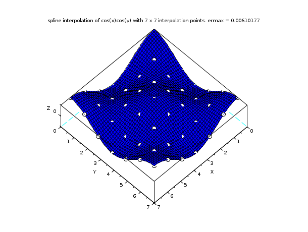
// example 1 : interpolation of cos(x)cos(y)
n = 7;  // a regular grid with n x n interpolation points
        // will be used
x = linspace(0,2*%pi,n); y = x;
z = cos(x')*cos(y);
C = splin2d(x, y, z, "periodic");
m = 50; // discretization parameter of the evaluation grid
xx = linspace(0,2*%pi,m); yy = xx;
[XX,YY] = ndgrid(xx,yy);
zz = interp2d(XX,YY, x, y, C);
emax = max(abs(zz - cos(xx')*cos(yy)));
clf()
plot3d(xx, yy, zz, flag=[2 4 4])
[X,Y] = ndgrid(x,y);
param3d1(X,Y,list(z,-9*ones(1,n)), flag=[0 0])
str = msprintf(" with %d x %d interpolation points. ermax = %g",n,n,emax)
xtitle("spline interpolation of cos(x)cos(y)"+str)
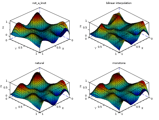
// example 2 : different interpolation functions on random data
n = 6;
x = linspace(0,1,n); y = x;
z = rand(n,n);
np = 50;
xp = linspace(0,1,np); yp = xp;
[XP, YP] = ndgrid(xp,yp);
ZP1 = interp2d(XP, YP, x, y, splin2d(x, y, z, "not_a_knot"));
ZP2 = linear_interpn(XP, YP, x, y, z);
ZP3 = interp2d(XP, YP, x, y, splin2d(x, y, z, "natural"));
ZP4 = interp2d(XP, YP, x, y, splin2d(x, y, z, "monotone"));
xset("colormap", jetcolormap(64))
clf()
subplot(2,2,1)
plot3d1(xp, yp, ZP1, flag=[2 2 4])
xtitle("not_a_knot")
subplot(2,2,2)
plot3d1(xp, yp, ZP2, flag=[2 2 4])
xtitle("bilinear interpolation")
subplot(2,2,3)
plot3d1(xp, yp, ZP3, flag=[2 2 4])
xtitle("natural")
subplot(2,2,4)
plot3d1(xp, yp, ZP4, flag=[2 2 4])
xtitle("monotone")
show_window()
// example 3 : not_a_knot spline and monotone sub-spline
//             on a step function
a = 0; b = 1; c = 0.25; d = 0.75;
// create interpolation grid
n = 11;
x = linspace(a,b,n);
ind = find(c <= x & x <= d);
z = zeros(n,n); z(ind,ind) = 1;  // a step inside a square
// create evaluation grid
np = 220;
xp = linspace(a,b, np);
[XP, YP] = ndgrid(xp, xp);
zp1 = interp2d(XP, YP, x, x, splin2d(x,x,z));
zp2 = interp2d(XP, YP, x, x, splin2d(x,x,z,"monotone"));
// plot
clf()
xset("colormap",jetcolormap(128))
subplot(1,2,1)
plot3d1(xp, xp, zp1, flag=[-2 6 4])
xtitle("spline (not_a_knot)")
subplot(1,2,2)
plot3d1(xp, xp, zp2, flag=[-2 6 4])
xtitle("subspline (monotone)")
See Also
- cshep2d — bidimensional cubic shepard (scattered) interpolation
- linear_interpn — n dimensional linear interpolation
- interp2d — bicubic spline (2d) evaluation function
History
| Версия | Описание |
| 5.4.0 | previously, imaginary part of input arguments were implicitly ignored. |
| Report an issue | ||
| << splin | Interpolation | splin3d >> |