Please note that the recommended version of Scilab is 2026.1.0. This page might be outdated.
See the recommended documentation of this function
splin
cubic spline interpolation
Calling Sequence
d = splin(x, y [,spline_type [, der]])
Arguments
- x
a strictly increasing (row or column) vector (x must have at least 2 components)
- y
a vector of same format than
x- spline_type
(optional) a string selecting the kind of spline to compute
- der
(optional) a vector with 2 components, with the end points derivatives (to provide when spline_type="clamped")
- d
vector of the same format than
x(diis the derivative of the spline atxi)
Description
This function computes a cubic spline or sub-spline
s which interpolates the (xi,yi)
points, ie, we have s(xi)=yi for all
i=1,..,n. The resulting spline s
is completely defined by the triplet (x,y,d) where
d is the vector with the derivatives at the
xi: s'(xi)=di (this is called the
Hermite form). The evaluation of the spline at some
points must be done by the interp function.
Several kind of splines may be computed by selecting the appropriate
spline_type parameter:
- "not_a_knot"
this is the default case, the cubic spline is computed by using the following conditions (considering n points x1,...,xn):

- "clamped"
in this case the cubic spline is computed by using the end points derivatives which must be provided as the last argument
der:
- "natural"
the cubic spline is computed by using the conditions:

- "periodic"
a periodic cubic spline is computed (
ymust verify y1=yn) by using the conditions:
- "monotone"
in this case a sub-spline (s is only one continuously differentiable) is computed by using a local scheme for the di such that s is monotone on each interval:

- "fast"
in this case a sub-spline is also computed by using a simple local scheme for the di : d(i) is the derivative at x(i) of the interpolation polynomial of (x(i-1),y(i-1)), (x(i),y(i)),(x(i+1),y(i+1)), except for the end points (d1 being computed from the 3 left most points and dn from the 3 right most points).
- "fast_periodic"
same as before but use also a centered formula for d1 = s'(x1) = dn = s'(xn) by using the periodicity of the underlying function (
ymust verify y1=yn).
Remarks
From an accuracy point of view use essentially the clamped type if you know the end point derivatives,
else use not_a_knot. But if the
underlying approximated function is periodic use the periodic type. Under the good assumptions these
kind of splines got an O(h^4) asymptotic behavior of
the error. Don't use the natural type
unless the underlying function have zero second end points
derivatives.
The monotone, fast (or fast_periodic) type may be useful in some cases,
for instance to limit oscillations (these kind of sub-splines have an
O(h^3) asymptotic behavior of the error).
If n=2 (and spline_type is
not clamped) linear interpolation is
used. If n=3 and spline_type is
not_a_knot, then a fast sub-spline type is in fact computed.
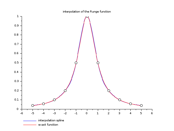
Examples
// example 1
deff("y=runge(x)","y=1 ./(1 + x.^2)")
a = -5; b = 5; n = 11; m = 400;
x = linspace(a, b, n)';
y = runge(x);
d = splin(x, y);
xx = linspace(a, b, m)';
yyi = interp(xx, x, y, d);
yye = runge(xx);
clf()
plot2d(xx, [yyi yye], style=[2 5], leg="interpolation spline@exact function")
plot2d(x, y, -9)
xtitle("interpolation of the Runge function")
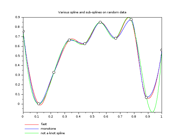
// example 2 : show behavior of different splines on random data
a = 0; b = 1;        // interval of interpolation
n = 10;              // nb of interpolation  points
m = 800;             // discretization for evaluation
x = linspace(a,b,n)'; // abscissae of interpolation points
y = rand(x);          // ordinates of interpolation points
xx = linspace(a,b,m)';
yk = interp(xx, x, y, splin(x,y,"not_a_knot"));
yf = interp(xx, x, y, splin(x,y,"fast"));
ym = interp(xx, x, y, splin(x,y,"monotone"));
clf()
plot2d(xx, [yf ym yk], style=[5 2 3], strf="121", ...
       leg="fast@monotone@not a knot spline")
plot2d(x,y,-9, strf="000")  // to show interpolation points
xtitle("Various spline and sub-splines on random data")
show_window()
See Also
History
| Версия | Описание |
| 5.4.0 | previously, imaginary part of input arguments were implicitly ignored. |
| Report an issue | ||
| << smooth | Interpolation | splin2d >> |