Please note that the recommended version of Scilab is 2026.1.0. This page might be outdated.
See the recommended documentation of this function
linear_interpn
n dimensional linear interpolation
Calling Sequence
vp = linear_interpn(xp1,xp2,..,xpn, x1, ..., xn, v [,out_mode])
Arguments
- xp1, xp2, .., xpn
real vectors (or matrices) of same size
- x1 ,x2, ..., xn
strictly increasing row vectors (with at least 2 components) defining the n dimensional interpolation grid
- v
vector (case n=1), matrix (case n=2) or hypermatrix (case n > 2) with the values of the underlying interpolated function at the grid points.
- out_mode
(optional) string defining the evaluation outside the grid (extrapolation)
- vp
vector or matrix of same size than
xp1, ...,
                            xpn
Description
Given a n dimensional grid defined by the n vectors x1 ,x2,
..., xn
and the values v of a function (says
f) at the grid points :

this function computes the linear interpolant of
f from the grid (called s in the
following) at the points which coordinates are defined by the vectors (or
matrices) xp1, xp2, ..., xpn:

The out_mode parameter set the evaluation rule
for extrapolation: if we note
Pi=(xp1(i),xp2(i),...,xpn(i)) then
out_mode defines the evaluation rule when:

The different choices are:
- "by_zero"
an extrapolation by zero is done
- "by_nan"
extrapolation by Nan
- "C0"
the extrapolation is defined as follows:
- "natural"
the extrapolation is done by using the nearest n-linear patch from the point.
- "periodic"
sis extended by periodicity.
Examples
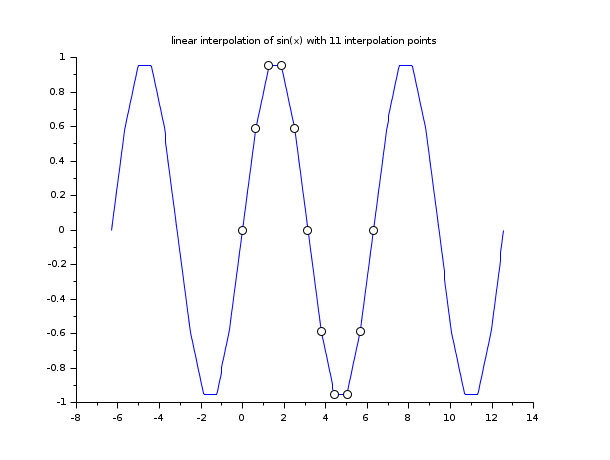
// example 1 : 1d linear interpolation
x = linspace(0,2*%pi,11);
y = sin(x);
xx = linspace(-2*%pi,4*%pi,400)';
yy = linear_interpn(xx, x, y, "periodic");
clf()
plot2d(xx,yy,style=2)
plot2d(x,y,style=-9, strf="000")
xtitle("linear interpolation of sin(x) with 11 interpolation points")
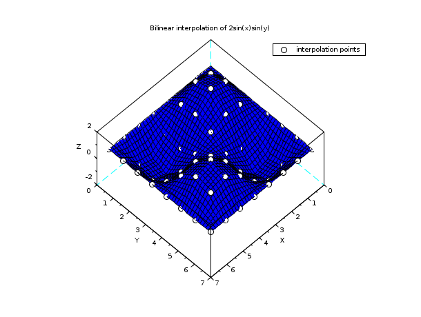
// example 2 : bilinear interpolation
n = 8;
x = linspace(0,2*%pi,n); y = x;
z = 2*sin(x')*sin(y);
xx = linspace(0,2*%pi, 40);
[xp,yp] = ndgrid(xx,xx);
zp = linear_interpn(xp,yp, x, y, z);
clf()
plot3d(xx, xx, zp, flag=[2 6 4])
[xg,yg] = ndgrid(x,x);
param3d1(xg,yg, list(z,-9*ones(1,n)), flag=[0 0])
xtitle("Bilinear interpolation of 2sin(x)sin(y)")
legends("interpolation points",-9,1)
show_window()
// example 3 : bilinear interpolation and experimentation
//             with all the outmode features
nx = 20; ny = 30;
x = linspace(0,1,nx);
y = linspace(0,2, ny);
[X,Y] = ndgrid(x,y);
z = 0.4*cos(2*%pi*X).*cos(%pi*Y);
nxp = 60 ; nyp = 120;
xp = linspace(-0.5,1.5, nxp);
yp = linspace(-0.5,2.5, nyp);
[XP,YP] = ndgrid(xp,yp);
zp1 = linear_interpn(XP, YP, x, y, z, "natural");
zp2 = linear_interpn(XP, YP, x, y, z, "periodic");
zp3 = linear_interpn(XP, YP, x, y, z, "C0");
zp4 = linear_interpn(XP, YP, x, y, z, "by_zero");
zp5 = linear_interpn(XP, YP, x, y, z, "by_nan");
clf()
subplot(2,3,1)
plot3d(x, y, z, leg="x@y@z", flag = [2 4 4])
xtitle("initial function 0.4 cos(2 pi x) cos(pi y)")
subplot(2,3,2)
plot3d(xp, yp, zp1, leg="x@y@z", flag = [2 4 4])
xtitle("Natural")
subplot(2,3,3)
plot3d(xp, yp, zp2, leg="x@y@z", flag = [2 4 4])
xtitle("Periodic")
subplot(2,3,4)
plot3d(xp, yp, zp3, leg="x@y@z", flag = [2 4 4])
xtitle("C0")
subplot(2,3,5)
plot3d(xp, yp, zp4, leg="x@y@z", flag = [2 4 4])
xtitle("by_zero")
subplot(2,3,6)
plot3d(xp, yp, zp5, leg="x@y@z", flag = [2 4 4])
xtitle("by_nan")
show_window()
// example 4 : trilinear interpolation (see splin3d help
//             page which have the same example with
//             tricubic spline interpolation)
exec("SCI/modules/interpolation/demos/interp_demo.sci");
func =  "v=(x-0.5).^2 + (y-0.5).^3 + (z-0.5).^2";
deff("v=f(x,y,z)",func);
n = 5;
x = linspace(0,1,n); y=x; z=x;
[X,Y,Z] = ndgrid(x,y,z);
V = f(X,Y,Z);
// compute (and display) the linear interpolant on some slices
m = 41;
dir = ["z="  "z="  "z="  "x="  "y="];
val = [ 0.1   0.5   0.9   0.5   0.5];
ebox = [0 1 0 1 0 1];

XF=[]; YF=[]; ZF=[]; VF=[];
for i = 1:length(val)
  [Xm,Xp,Ym,Yp,Zm,Zp] = slice_parallelepiped(dir(i), val(i), ebox, m, m, m);
  Vm = linear_interpn(Xm,Ym,Zm, x, y, z, V);
  [xf,yf,zf,vf] = nf3dq(Xm,Ym,Zm,Vm,1);
  XF = [XF xf]; YF = [YF yf]; ZF = [ZF zf]; VF = [VF vf];
  Vp =  linear_interpn(Xp,Yp,Zp, x, y, z, V);
  [xf,yf,zf,vf] = nf3dq(Xp,Yp,Zp,Vp,1);
  XF = [XF xf]; YF = [YF yf]; ZF = [ZF zf]; VF = [VF vf];
end
nb_col = 128;
vmin = min(VF); vmax = max(VF);
color = dsearch(VF,linspace(vmin,vmax,nb_col+1));
xset("colormap",jetcolormap(nb_col));
clf()
xset("hidden3d",xget("background"))
colorbar(vmin,vmax)
plot3d(XF, YF, list(ZF,color), flag=[-1 6 4])
xtitle("tri-linear interpolation of "+func)
show_window()
See Also
History
| Версия | Описание |
| 5.4.0 | previously, imaginary part of input arguments were implicitly ignored. |
| Report an issue | ||
| << interpln | Interpolation | lsq_splin >> |