Please note that the recommended version of Scilab is 2026.1.0. This page might be outdated.
See the recommended documentation of this function
plot3d
3D plot of a surface
Calling Sequence
plot3d(x,y,z,[theta,alpha,leg,flag,ebox])
plot3d(x,y,z,<opt_args>)

plot3d(xf,yf,zf,[theta,alpha,leg,flag,ebox])
plot3d(xf,yf,zf,<opt_args>)

plot3d(xf,yf,list(zf,colors),[theta,alpha,leg,flag,ebox])
plot3d(xf,yf,list(zf,colors),<opt_args>)

plot3d(z)
Arguments
- x,y
row vectors of sizes n1 and n2 (x-axis and y-axis coordinates). These coordinates must be monotone.
- z
matrix of size (n1,n2).
z(i,j)is the value of the surface at the point (x(i),y(j)).- xf,yf,zf
matrices of size (nf,n). They define the facets used to draw the surface. There are
nfacets. Each facetiis defined by a polygon withnfpoints. The x-axis, y-axis and z-axis coordinates of the points of the ith facet are given respectively byxf(:,i),yf(:,i)andzf(:,i).- colors
a vector of size n giving the color of each facets or a matrix of size (nf,n) giving color near each facet boundary (facet color is interpolated ).
- <opt_args>
This represents a sequence of statements
key1=value1,
                            key2=value2
,... wherekey1,key2,...can be one of the following: theta, alpha ,leg,flag,ebox (see definition below).- theta, alpha
real values giving in degree the spherical coordinates of the observation point (by default,
alpha=35° andtheta=45°).- leg
string defining the labels for each axis with @ as a field separator, for example "X@Y@Z" (by default, axis have no label).
- flag
a real vector of size three.
flag=[mode,type,box](by defaultflag=[2,8,4]).- mode
an integer (surface color).
- mode>0
the surface is painted with color
"mode"; the boundary of the facet is drawn with current line style and color.- mode=0:
a mesh of the surface is drawn.
- mode<0:
the surface is painted with color
"-mode"; the boundary of the facet is not drawn.Note that the surface color treatement can be done using
color_modeandcolor_flagoptions through the surface entity properties (see surface_properties).
- type
an integer (scaling).
- type=0:
the plot is made using the current 3D scaling (set by a previous call to
param3d,plot3d,contourorplot3d1).- type=1:
rescales automatically 3d boxes with extreme aspect ratios, the boundaries are specified by the value of the optional argument
ebox.- type=2:
rescales automatically 3d boxes with extreme aspect ratios, the boundaries are computed using the given data.
- type=3:
3d isometric with box bounds given by optional
ebox, similarily totype=1.- type=4:
3d isometric bounds derived from the data, to similarily
type=2.- type=5:
3d expanded isometric bounds with box bounds given by optional
ebox, similarily totype=1.- type=6:
3d expanded isometric bounds derived from the data, similarily to
type=2.Note that axes boundaries can be customized through the axes entity properties (see axes_properties).
- box
an integer (frame around the plot).
- box=0:
nothing is drawn around the plot.
- box=1:
unimplemented (like box=0).
- box=2:
only the axes behind the surface are drawn.
- box=3:
a box surrounding the surface is drawn and captions are added.
- box=4:
a box surrounding the surface is drawn, captions and axes are added.
Note that axes aspect can also be customized through the axes entity properties (see axes_properties).
- ebox
It specifies the boundaries of the plot as the vector
[xmin,xmax,ymin,ymax,zmin,zmax]. This argument is used together withtypeinflag: if it is set to1,3or5(see above to see the corresponding behaviour). Ifflagis missing,eboxis not taken into acoount (by defaulteboxis missing).Note that, when specified, the
eboxargument acts on thedata_boundsfield that can also be reset through the axes entity properties (see axes_properties).
Description
plot3d(z) draws the parametric surface z=f(x,y) where
x=1:m, y=1:n and [m,n]=size(z).
plot3d(x,y,z,[theta,alpha,leg,flag,ebox]) draws
the parametric surface z=f(x,y).
plot3d(xf,yf,zf,[theta,alpha,leg ,flag,ebox])
draws a surface defined by a set of facets. You can draw multiple plots by
replacing xf, yf and
zf by multiple matrices assembled by rows as
[xf1 xf2 ...], [yf1 yf2 ...] and
[zf1 zf2 ...]. Note that data can also be set or get
through the surface entity properties (see surface_properties).
You can give a specific color for each facet by using
list(zf,colors) instead of zf, where
colors is a vector of size n. If
colors(i) is positive it gives the color of facet
i and the boundary of the facet is drawn with current
line style and color. If colors(i) is negative, color
id -colors(i) is used and the boundary of the facet is
not drawn.
It is also possible to get interpolated color for facets. For that
the color argument must be a matrix of size nfxn giving the color near
each boundary of each facets. In this case positive values for colors mean
that the boundary are not drawn. Note that colors can also be set through
the surface entity properties (via tlist affectations)
and edited using color_flag option (see surface_properties).
The optional arguments theta, alpha, leg ,flag,
ebox
,can be passed by a sequence of statements
key1=value1, key2=value2, ... In this case, the order
has no special meaning. Note that all these optional arguments except
flag can be customized through the axes entity
properties (see axes_properties).
As described before, the flag option deals with surface
entity properties for mode (see surface_properties) and axes
properties for type and box (see
axes_properties).
You can use the function genfac3d to compute four
sided facets from the surface z=f(x,y).
eval3dp can also be used.
Enter the command plot3d() to see a demo.
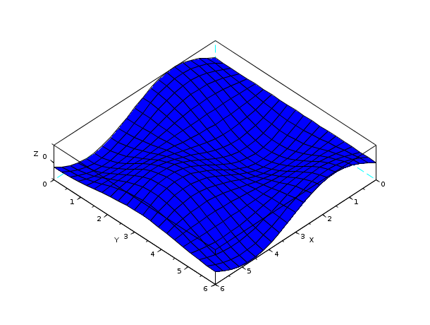
Examples
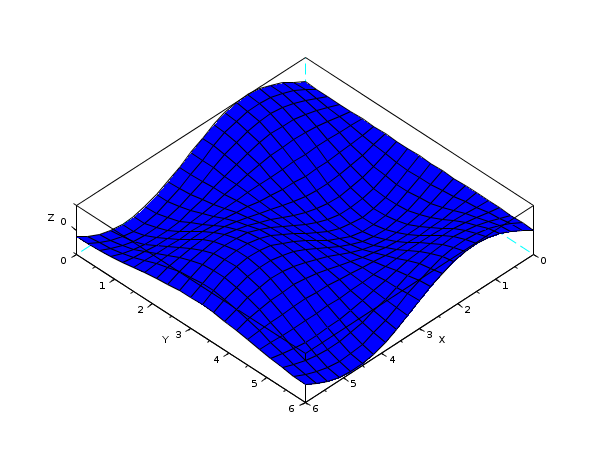
t=[0:0.3:2*%pi]';
z=sin(t)*cos(t');
// same plot using facets computed by genfac3d
[xx,yy,zz]=genfac3d(t,t,z);
plot3d(xx,yy,zz)
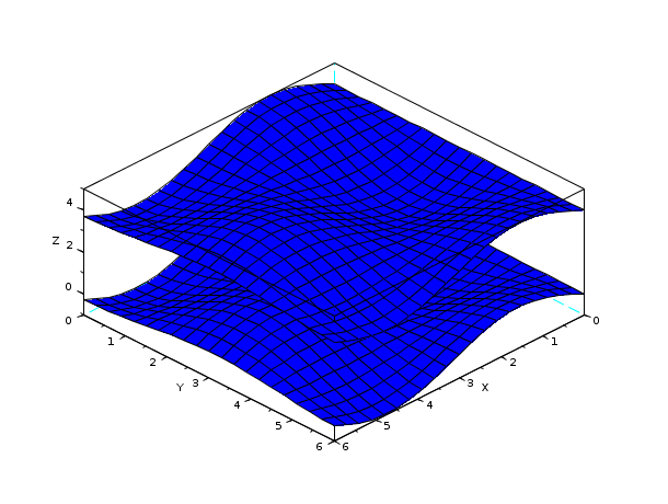
// multiple plots
t=[0:0.3:2*%pi]';
z=sin(t)*cos(t');
// same plot using facets computed by genfac3d
[xx,yy,zz]=genfac3d(t,t,z);
plot3d([xx xx],[yy yy],[zz 4+zz])
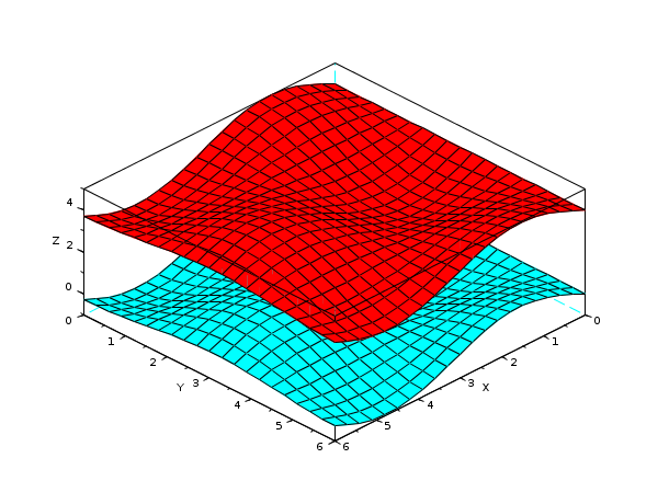
// multiple plots using colors
t=[0:0.3:2*%pi]';
z=sin(t)*cos(t');
// same plot using facets computed by genfac3d
[xx,yy,zz]=genfac3d(t,t,z);
plot3d([xx xx],[yy yy],list([zz zz+4],[4*ones(1,400) 5*ones(1,400)]))
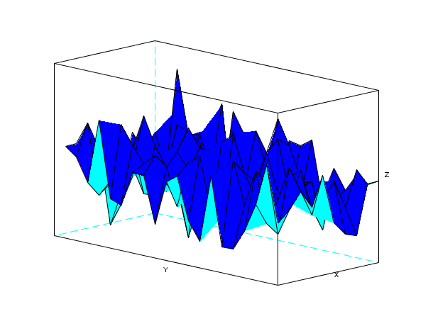
// simple plot with viewpoint and captions
plot3d(1:10,1:20,10*rand(10,20),alpha=35,theta=45,flag=[2,2,3])
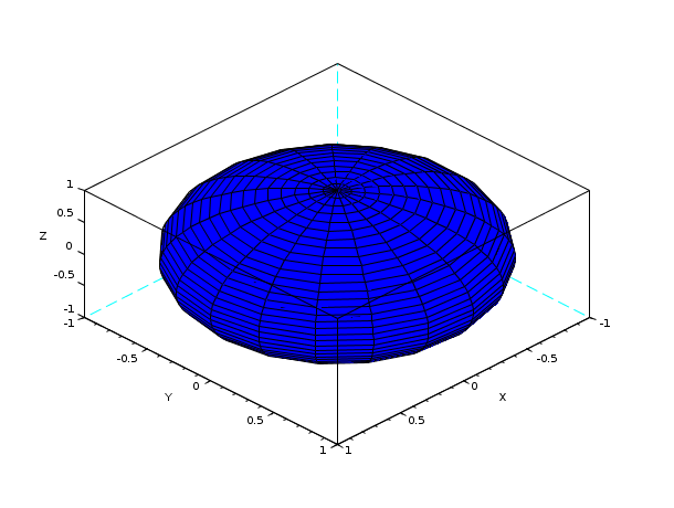
// plot of a sphere using facets computed by eval3dp
deff("[x,y,z]=sph(alp,tet)",["x=r*cos(alp).*cos(tet)+orig(1)*ones(tet)";..
     "y=r*cos(alp).*sin(tet)+orig(2)*ones(tet)";..
     "z=r*sin(alp)+orig(3)*ones(tet)"]);
r=1; orig=[0 0 0];
[xx,yy,zz]=eval3dp(sph,linspace(-%pi/2,%pi/2,40),linspace(0,%pi*2,20));
clf();plot3d(xx,yy,zz)
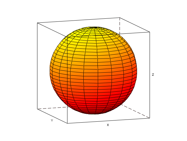
f=gcf();
f.color_map = hotcolormap(128);
r=0.3;orig=[1.5 0 0];
deff("[x,y,z]=sph(alp,tet)",["x=r*cos(alp).*cos(tet)+orig(1)*ones(tet)";..
     "y=r*cos(alp).*sin(tet)+orig(2)*ones(tet)";..
     "z=r*sin(alp)+orig(3)*ones(tet)"]);
[xx,yy,zz]=eval3dp(sph,linspace(-%pi/2,%pi/2,40),linspace(0,%pi*2,20));
[xx1,yy1,zz1]=eval3dp(sph,linspace(-%pi/2,%pi/2,40),linspace(0,%pi*2,20));
cc=(xx+zz+2)*32;cc1=(xx1-orig(1)+zz1/r+2)*32;
clf();plot3d1([xx xx1],[yy yy1],list([zz,zz1],[cc cc1]),theta=70,alpha=80,flag=[5,6,3])
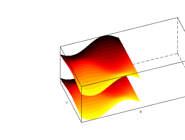
t=[0:0.3:2*%pi]'; z=sin(t)*cos(t');
[xx,yy,zz]=genfac3d(t,t,z);
plot3d([xx xx],[yy yy],list([zz zz+4],[4*ones(1,400) 5*ones(1,400)]))
e=gce();
f=e.data;
TL = tlist(["3d" "x" "y" "z" "color"],f.x,f.y,f.z,6*rand(f.z)); // random color matrix
e.data = TL;
TL2 = tlist(["3d" "x" "y" "z" "color"],f.x,f.y,f.z,4*rand(1,800)); // random color vector
e.data = TL2;
TL3 = tlist(["3d" "x" "y" "z" "color"],f.x,f.y,f.z,[20*ones(1,400) 6*ones(1,400)]);
e.data = TL3;
TL4 = tlist(["3d" "x" "y" "z"],f.x,f.y,f.z); // no color
e.data = TL4;
e.color_flag=1 // color index proportional to altitude (z coord.)
e.color_flag=2; // back to default mode
e.color_flag= 3; // interpolated shading mode (based on blue default color)
clf()
plot3d([xx xx],[yy yy],list([zz zz+4],[4*ones(1,400) 5*ones(1,400)]))
h=gce(); //get handle on current entity (here the surface)
a=gca(); //get current axes
a.rotation_angles=[40,70];
a.grid=[1 1 1]; //make grids
a.data_bounds=[-6,0,-1;6,6,5];
a.axes_visible="off"; //axes are hidden
a.axes_bounds=[.2 0 1 1];
h.color_flag=1; //color according to z
h.color_mode=-2;  //remove the facets boundary by setting color_mode to white color
h.color_flag=2; //color according to given colors
h.color_mode = -1; // put the facets boundary back by setting color_mode to black color
f=gcf();//get the handle of the parent figure
f.color_map=hotcolormap(512);
c=[1:400,1:400];
TL.color = [c;c+1;c+2;c+3];
h.data = TL;
h.color_flag=3; // interpolated shading mode
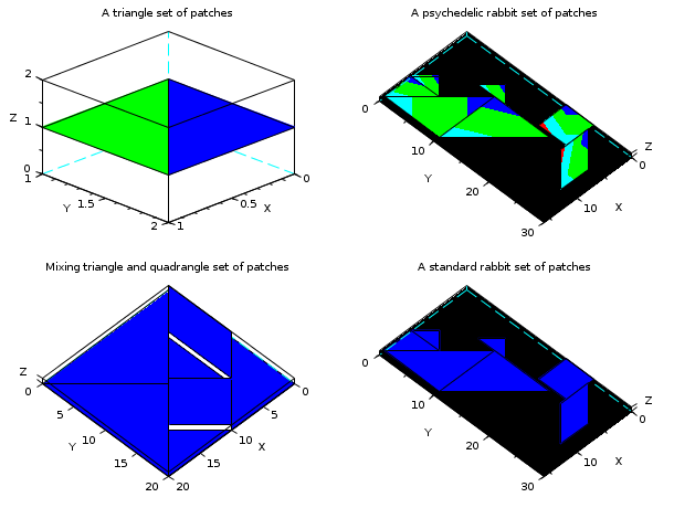
We can use the plot3d function to plot a set of patches (triangular, quadrangular, etc).
// The plot3d function to draw patches:
// patch(x,y,[z])
// patch(x,y,[list(z,c)])
// The size of x : number of points in the patches x number of patches
// y and z have the same sizes as x
// c:
// - a vector of size number of patches: the color of the patches
// - a matrix of size number of points in the patches x number of
//   patches: the color of each points of each patches

// Example 1: a set of triangular patches

x = [0 0;
     0 1;
     1 1];

y = [1 1;
     2 2;
     2 1];

z = [1 1;
     1 1;
     1 1];

tcolor = [2 3]';

subplot(2,2,1);
plot3d(x,y,list(z,tcolor));
xtitle('A triangle set of patches');
// Example 2: a mixture of triangular and quadrangular patches

xquad = [5, 0;
         10,0;
         15,5;
         10,5];

yquad = [15,0;
         20,10;
         15,15;
         10,5];

zquad = ones(4,2);

xtri = [ 0,10,10, 5, 0;
        10,20,20, 5, 0;
        20,20,15,10,10];

ytri = [ 0,10,20, 5,10;
        10,20,20,15,20;
         0, 0,15,10,20];

ztri = zeros(3,5);

subplot(2,2,3);
plot3d(xquad,yquad,zquad);
plot3d(xtri,ytri,ztri);
xtitle('Mixing triangle and quadrangle set of patches');

// Example 3: some rabbits

rabxtri = [ 5,  5, 2.5,  7.5, 10;
            5, 15, 5,   10,   10;
           15, 15, 5,   10,   15];

rabytri = [10, 10, 9.5,  2.5, 0;
           20, 10, 12,   5,   5;
           10   0   7    0    0];
rabztri = [0,0,0,0,0;
           0,0,0,0,0;
           0,0,0,0,0];

rabtricolor_byface = [2 2 2 2 2];

rabtricolor = [2,2,2,2,2;
               3,3,3,3,3;
               4,4,4,4,4];

rabxquad = [0, 1;
            0, 6;
            5,11;
            5, 6];

rabyquad = [18,23;
            23,28;
            23,28;
            18,23];

rabzquad = [1,1;
            1,1;
            1,1;
            1,1];

rabquadcolor_byface = [2 2];

rabquadcolor = [2,2;
                3,3;
                4,4;
                5,5];

subplot(2,2,2);
plot3d(rabxtri, rabytri, list(rabztri,rabtricolor));
plot3d(rabxquad,rabyquad,list(rabzquad,rabquadcolor));
h = gcf();
h.children(1).background = 1;
xtitle('A psychedelic rabbit set of patches');

subplot(2,2,4);
plot3d(rabxtri, rabytri, list(rabztri,rabtricolor_byface));
plot3d(rabxquad,rabyquad,list(rabzquad,rabquadcolor_byface));
h = gcf();
h.children(1).background = 1;
xtitle('A standard rabbit set of patches');
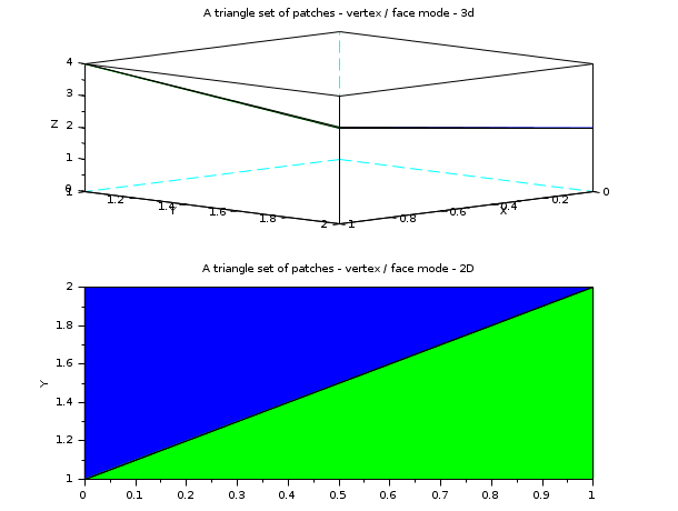
We can also use the plot3d function to plot a set of patches using vertex and faces.
// Vertex / Faces example: 3D example

// The vertex list contains the list of unique points composing each patch
// The points common to 2 patches are not repeated in the vertex list

vertex = [0 1 1;
          0 2 2;
          1 2 3;
          1 1 4];

// The face list indicates which points are composing the patch.
face = [1 2 3;
        1 3 4];

tcolor = [2 3]';

// The formula used to translate the vertex / face representation into x, y, z lists

xvf = matrix(vertex(face,1),size(face,1),length(vertex(face,1))/size(face,1))';
yvf = matrix(vertex(face,2),size(face,1),length(vertex(face,1))/size(face,1))';
zvf = matrix(vertex(face,3),size(face,1),length(vertex(face,1))/size(face,1))';

scf();
subplot(2,1,1);
plot3d(xvf,yvf,list(zvf,tcolor));
xtitle('A triangle set of patches - vertex / face mode - 3d');

// 2D test
// We use the 3D representation with a 0 Z values and then switch to 2D representation

// Vertex / Faces example: 3D example

// The vertex list contains the list of unique points composing each patch
// The points common to 2 patches are not repeated in the vertex list

vertex = [0 1;
          0 2;
          1 2;
          1 1];

// The face list indicates which points are composing the patch.
face = [1 2 3;
        1 3 4];

// The formula used to translate the vertex / face representation into x, y, z lists

xvf = matrix(vertex(face,1),size(face,1),length(vertex(face,1))/size(face,1))';
yvf = matrix(vertex(face,2),size(face,1),length(vertex(face,1))/size(face,1))';
zvf = matrix(zeros(vertex(face,2)),size(face,1),length(vertex(face,1))/size(face,1))';
tcolor = [2 3]';

subplot(2,1,2);
plot3d(xvf,yvf,list(zvf,tcolor));
xtitle('A triangle set of patches - vertex / face mode - 2D');
a = gca();
a.view = '2d';
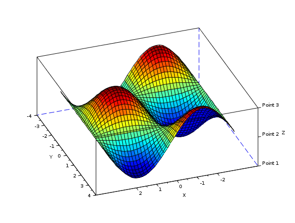
How to set manually some ticks
plot3d();
h = gca();
h.x_ticks = tlist(['ticks','locations','labels'],[-2,-1,0,1,2],['-2','-1','0','1','2']);
h.y_ticks = tlist(['ticks','locations','labels'],[-4,-3,-2,-1,0,1,2,3,4],['-4','-3','-2','-1','0','1','2','3','4']);
h.z_ticks = tlist(['ticks','locations','labels'],[-1,0,1],['Point 1','Point 2','Point 3']);
See Also
- eval3dp — compute facets of a 3D parametric surface
- genfac3d — Compute facets of a 3D surface
- geom3d — projection from 3D on 2D after a 3D plot
- param3d — 3D plot of a parametric curve
- plot3d1 — 3D gray or color level plot of a surface
- clf — Clear or reset or reset a figure or a frame uicontrol.
- gca — Return handle of current axes.
- gcf — Return handle of current graphic window.
- xdel — удаление графического окна
- delete — delete a graphic entity and its children.
- axes_properties — description of the axes entity properties
| Report an issue | ||
| << param3d properties | 3d_plot | plot3d1 >> |