- Scilab Help
- CACSD (Computer Aided Control Systems Design)
- Formal representations and conversions
- Plot and display
- abinv
- arhnk
- arl2
- arma
- arma2p
- arma2ss
- armac
- armax
- armax1
- arsimul
- augment
- balreal
- bilin
- bstap
- cainv
- calfrq
- canon
- ccontrg
- cls2dls
- colinout
- colregul
- cont_mat
- contr
- contrss
- copfac
- csim
- ctr_gram
- damp
- dcf
- ddp
- dhinf
- dhnorm
- dscr
- dsimul
- dt_ility
- dtsi
- equil
- equil1
- feedback
- findABCD
- findAC
- findBD
- findBDK
- findR
- findx0BD
- flts
- fourplan
- freq
- freson
- fspec
- fspecg
- fstabst
- g_margin
- gamitg
- gcare
- gfare
- gfrancis
- gtild
- h2norm
- h_cl
- h_inf
- h_inf_st
- h_norm
- hankelsv
- hinf
- imrep2ss
- inistate
- invsyslin
- kpure
- krac2
- lcf
- leqr
- lft
- lin
- linf
- linfn
- linmeq
- lqe
- lqg
- lqg2stan
- lqg_ltr
- lqr
- ltitr
- macglov
- minreal
- minss
- mucomp
- narsimul
- nehari
- noisegen
- nyquistfrequencybounds
- obs_gram
- obscont
- observer
- obsv_mat
- obsvss
- p_margin
- parrot
- pfss
- phasemag
- plzr
- pol2des
- ppol
- prbs_a
- projsl
- repfreq
- ric_desc
- ricc
- riccati
- routh_t
- rowinout
- rowregul
- rtitr
- sensi
- sident
- sorder
- specfact
- ssprint
- st_ility
- stabil
- sysfact
- syslin
- syssize
- time_id
- trzeros
- ui_observer
- unobs
- zeropen
Please note that the recommended version of Scilab is 2026.1.0. This page might be outdated.
See the recommended documentation of this function
calfrq
frequency response discretization
Calling Sequence
[frq,bnds,split]=calfrq(h,fmin,fmax)
Arguments
- h
Linear system in state space or transfer representation (
see syslin)- fmin,fmax
real scalars (min and max frequencies in Hz)
- frq
row vector (discretization of the frequency interval)
- bnds
vector
[Rmin Rmax Imin Imax]whereRminandRmaxare the lower and upper bounds of the frequency response real part,IminandImaxare the lower and upper bounds of the frequency response imaginary part,- split
vector of frq splitting points indexes
Description
frequency response discretization; frq is the
discretization of [fmin,fmax] such that the peaks in
the frequency response are well represented.
Singularities are located between frq(split(k)-1)
and frq(split(k)) for k>1.
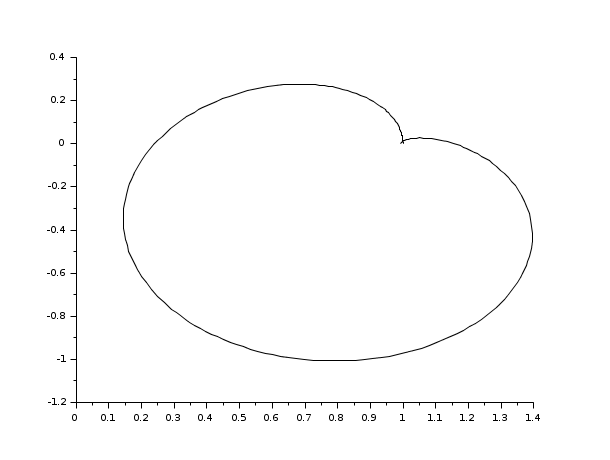
Examples
s=poly(0,'s')
h=syslin('c',(s^2+2*0.9*10*s+100)/(s^2+2*0.3*10.1*s+102.01))
h1=h*syslin('c',(s^2+2*0.1*15.1*s+228.01)/(s^2+2*0.9*15*s+225))
[f1,bnds,spl]=calfrq(h1,0.01,1000);
rf=repfreq(h1,f1);
plot2d(real(rf)',imag(rf)')
See Also
| Report an issue | ||
| << cainv | CACSD (Computer Aided Control Systems Design) | canon >> |