- Scilab help
- CACSD (Computer Aided Control Systems Design)
- Formal representations and conversions
- Plot and display
- abinv
- arhnk
- arl2
- arma
- arma2p
- arma2ss
- armac
- armax
- armax1
- arsimul
- augment
- balreal
- bilin
- bstap
- cainv
- calfrq
- canon
- ccontrg
- cls2dls
- colinout
- colregul
- cont_mat
- contr
- contrss
- copfac
- csim
- ctr_gram
- damp
- dcf
- ddp
- dhinf
- dhnorm
- dscr
- dsimul
- dt_ility
- dtsi
- equil
- equil1
- feedback
- findABCD
- findAC
- findBD
- findBDK
- findR
- findx0BD
- flts
- fourplan
- freq
- freson
- fspec
- fspecg
- fstabst
- g_margin
- gamitg
- gcare
- gfare
- gfrancis
- gtild
- h2norm
- h_cl
- h_inf
- h_inf_st
- h_norm
- hankelsv
- hinf
- imrep2ss
- inistate
- invsyslin
- kpure
- krac2
- lcf
- leqr
- lft
- lin
- linf
- linfn
- linmeq
- lqe
- lqg
- lqg2stan
- lqg_ltr
- lqr
- ltitr
- macglov
- minreal
- minss
- mucomp
- narsimul
- nehari
- noisegen
- nyquistfrequencybounds
- obs_gram
- obscont
- observer
- obsv_mat
- obsvss
- p_margin
- parrot
- pfss
- phasemag
- plzr
- pol2des
- ppol
- prbs_a
- projsl
- reglin
- repfreq
- ric_desc
- ricc
- riccati
- routh_t
- rowinout
- rowregul
- rtitr
- sensi
- sident
- sorder
- specfact
- ssprint
- st_ility
- stabil
- sysfact
- syslin
- syssize
- time_id
- trzeros
- ui_observer
- unobs
- zeropen
Please note that the recommended version of Scilab is 2026.1.0. This page might be outdated.
See the recommended documentation of this function
damp
Natural frequencies and damping factors.
Calling Sequence
[wn,z] = damp(sys)
[wn,z] = damp(P [,dt])
[wn,z] = damp(R [,dt])
Parameters
- sys
A linear dynamical system (see syslin).
- P
An array of polynomials.
- P
An array of real or complex floating point numbers.
- dt
A non negative scalar, with default value 0.
- wn
vector of floating point numbers in increasing order: the natural pulsation in rd/s.
- z
vector of floating point numbers: the damping factors.
Description
The denominator second order continuous time transfer function
with complex poles can be written as s^2+2*z*wn*s+wn^2 wherez
is the damping factor and wnthe natural pulsation.
If sys is a continuous time system,
[wn,z] = damp(sys) returns in wn the natural
pulsation  (in rd/s) and in
 z the damping factors
 of the poles of the linear dynamical system
sys. The wn and
z arrays are ordered according to the increasing
pulsation order.
If sys is a discrete time system
[wn,z] = damp(sys) returns in
wn the natural pulsation
 (in rd/s) and in
 z the
damping factors  of the continuous time
equivalent poles of
of the continuous time
equivalent poles of sys. The
wn and z arrays are
ordered according to the increasing pulsation order.
[wn,z] = damp(P) returns in
wn the natural pulsation
 (in rd/s) and in
 z the
damping factors  of the set of roots of the polynomials
stored in the
of the set of roots of the polynomials
stored in the P array. If
dt is given and non 0, the roots are first
converted to their continuous time equivalents.
The wn and z arrays are ordered
according to the increasing pulsation order.
[wn,z] = damp(R) returns in
wn the natural pulsation
 (in rd/s) and in
 z the
damping factors  of the set of roots stored in the
R array.
If dt is given and non 0, the roots are first
converted to their continuous time equivalents.
wn(i) and z(i) are the the
natural pulsation and damping factor of R(i).
Examples
s=%s;
num=22801+4406.18*s+382.37*s^2+21.02*s^3+s^4;
den=22952.25+4117.77*s+490.63*s^2+33.06*s^3+s^4
h=syslin('c',num/den);
[wn,z] = damp(h)
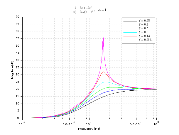
The following example illustrates the effect of the damping factor on the frequency response of a second order system.
s=%s;
wn=1;
clf();
Z=[0.95 0.7 0.5 0.3 0.13 0.0001];
for k=1:size(Z,'*')
  z=Z(k)
  H=syslin('c',1+5*s+10*s^2,s^2+2*z*wn*s+wn^2);
  gainplot(H,0.01,1)
  p=gce();p=p.children;
  p.foreground=k;
end
title("$\frac{1+5 s+10 s^2}{\omega_n^2+2\omega_n\xi s+s^2}, \quad \omega_n=1$")
legend('$\xi='+string(Z)+'$')
plot(wn/(2*%pi)*[1 1],[0 70],'r') //natural pulsation
Computing the natural pulsations and daping ratio for a set of roots:
[wn,z] = damp((1:5)+%i)
| Report an issue | ||
| << ctr_gram | CACSD (Computer Aided Control Systems Design) | dcf >> |