nyquist

Arguments

sl

a continuous or discrete time SIMO linear dynamical system ( see: syslin).

fmin,fmax

real scalars (frequency bounds (in Hz))

step

real (logarithmic discretization step)

comments

string vector (captions).

frq

vector or matrix of frequencies (in Hz) (one row for each output of sl).

db,phi

real matrices of modulus (in dB) and phases (in degree) (one row for each output of sl).

repf

matrix of complex numbers. Frequency response (one row for aech output of sl)

Description

Nyquist plot i.e Imaginary part versus Real part of the frequency response of sl.

For continuous time systems sl(2*%i*%pi*w) is plotted. For discrete time system or discretized systems sl(exp(2*%i*%pi*w*fd) is used ( fd=1 for discrete time systems and fd=sl('dt') for discretized systems )

sl can be a continuous-time or discrete-time SIMO system (see syslin). In case of multi-output the outputs are plotted with different symbols.

The frequencies are given by the bounds fmin,fmax (in Hz) or by a row-vector (or a matrix for multi-output) frq.

step is the ( logarithmic ) discretization step. (see calfrq for the choice of default value).

comments is a vector of character strings (captions).

db,phi are the matrices of modulus (in Db) and phases (in degrees). (One row for each response).

repf is a matrix of complex numbers. One row for each response.

Default values for fmin and fmax are 1.d-3, 1.d+3 if sl is continuous-time or 1.d-3, 0.5/sl.dt (nyquist frequency) if sl is discrete-time.

Automatic discretization of frequencies is made by calfrq.

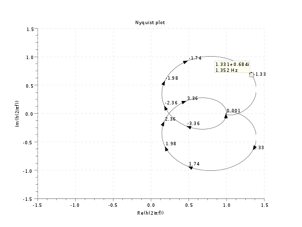
To obtain the value of the frequency at a selected point(s) you can activate the datatips manager and click the desired point on the nyquist curve(s).

Graphics entities organization

The nyquist function creates a compound object for each SISO system. The following piece of code allows to get the handle on the compound object of the ith system:

ax=gca();//handle on current axes
hi=ax.children($+i-1)// the handle on the compound object of the ith system

This compound object has two children: a compound object that defines the small arrows (a compound of small polylines) and the curve labels (a compound of texts) and a polyline which is the curve itself. The following piece of code shows how one can customize a particular nyquist curve display.

hi.children(1).visible='off'; //hides the arrows and labels
hi.children(2).thickness=2; //make the curve thicker

Examples

//Nyquist curve
s=poly(0,'s')
h=syslin('c',(s^2+2*0.9*10*s+100)/(s^2+2*0.3*10.1*s+102.01));
h1=h*syslin('c',(s^2+2*0.1*15.1*s+228.01)/(s^2+2*0.9*15*s+225))
clf();    nyquist(h1)
// add a datatip
ax=gca();
h_h=ax.children($).children(2);//handle on Nyquist curve of h
tip=datatipCreate(h_h,[1.331,0.684]);
datatipSetOrientation(tip,"upper left");

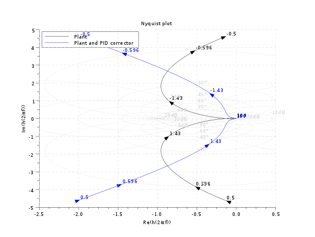
//Hall chart as a grid for nyquist
s=poly(0,'s');
Plant=syslin('c',16000/((s+1)*(s+10)*(s+100)));
//two degree of freedom PID
tau=0.2;xsi=1.2;
PID=syslin('c',(1/(2*xsi*tau*s))*(1+2*xsi*tau*s+tau^2*s^2));
clf();
nyquist([Plant;Plant*PID],0.5,100,["Plant";"Plant and PID corrector"]);
hallchart(colors=color('light gray')*[1 1])
//move the caption in the lower rigth corner
ax=gca();Leg=ax.children(1);
Leg.legend_location="in_upper_left";

See Also

• syslin — linear system definition
• bode — Bode plot
• black — Black-Nichols diagram of a linear dynamical system
• calfrq — frequency response discretization
• freq — frequency response
• repfreq — frequency response
• phasemag — phase and magnitude computation
• datatips — Tool for placing and editing tips along the plotted curves.