Please note that the recommended version of Scilab is 2026.1.0. This page might be outdated.
See the recommended documentation of this function
mapsound
Computes and displays an Amplitude(time, frequency) spectrogram of a sound record
Syntax
mapsound(signal)
mapsound(signal, Dt)
mapsound(signal, Dt, freqRange)
mapsound(signal, Dt, freqRange, samplingRate)
mapsound(signal, Dt, freqRange, samplingRate, Colormap)
data = mapsound(…)
Arguments
- signal
- Vector or matrix of signed real numbers representing the sound signal. If it's a matrix, its smallest size is considered as the number of channels. Then, only the first channel is considered and mapped.
- samplingRate
- Positive decimal number: Value of the sampling rate of the input
signal, in Hz. 22050 Hz is the default rate. - freqRange
- Specifies the interval [fmin, fmax] of positive sound frequencies to be
analyzed and mapped:
- If it's a scalar: It specifies the upper bound
fmax. Thenfmin=0is used. - If it's a vector: It specifies [fmin, fmax].
[0, 0.2*samplingRate]. - If it's a scalar: It specifies the upper bound
- Dt
- Specifies the time step of the map. The time step is also the
duration of each sound chunk considered at every time step, since the
signalis sliced into contiguous chunks without overlap. - data
- Structure with 3 fields returning values of computed and plotted data:
- times: Vector of mapped times, in seconds.
- frequencies: Vector of mapped frequencies, in Hz.
- amplitudes: Matrix of mapped absolute spectral amplitudes, of size length(.frequencies)×length(.times).
- Colormap
- Identifier of the colormap function to use: autumncolormap, bonecolormap, etc. The actual colormap is based on and built with it, but is not equal to it. It can be inverted in order to get light colors for low amplitudes, and be extrapolated to white if it does not natively include light colors.
Description
mapsound(…) slices the input signal in consecutive chunks #0, #1,.. of equal duration
Dt, up to the end of the signal. Then a discrete Fourier Transform
is computed for each chunk. The absolute value of the spectral amplitude of the chunk
#i is displayed at the time i*Dt, for frequencies in the chosen interval.
When Dt is not specified, mapsound(…) computes it in order to have
(almost) the same number of frequency and time bins, with the highest possible
(time, frequency) resolution. We may keep in mind that both time Dt
and frequency Δf steps are linked together by Dt.Δf=1. Thus, improving
one of both automatically alters the other one.
The (time, frequency, amplitude) values of any pixel are relative to its lower left corner. The time is at the beginning of the chunk. Amplitudes are given in the same unit and scale than for the input signal.
When the map is drawn in a new figure or a new axes alone in the figure,
a smart colormap is created and assigned to the figure and used for the map.
A colobar is displayed anyway. The number of frequency and time bins are
displayed below the bar. The default grid color is extracted from the sound map
colormap. xgrid(0) may be used to get a more visible black grid.
Most of input arguments are optional. To skip an argument and use its default value, just omit it before the next coma. [] used as default value works as well.
Examples
Example #1: A sound made of 2 pure sine waves of known amplitudes and frequencies is considered:
// Let's build the sound
// 1 s at 800 Hz @ amplitude=1.5, then 1 s at 1200 Hz @ amplitude = 1:
fs = 22050;
t = 0:1/fs:1*(1-%eps);
y = 0.3 + [1.5*sin(2*%pi*800*t) sin(2*%pi*1200*t)];

// Let's hear it:
playsnd(y/4)

// Then: build and display its map:
clf
mapsound(y, 0.04, 1500)
title "0.3 + [1.5⋅sin(2π⋅800⋅t), sin(2π⋅1200⋅t)]" fontsize 3.2
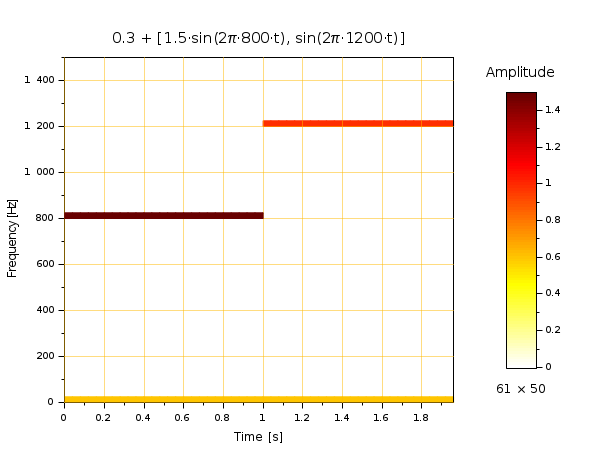
Both frequencies and amplitudes values are reliably mapped, as well as the average level, with the 2×0.3 amplitude at the zero frequency.
Example #2: Amplitude modulation: A Fc=1000 Hz carrier frequency is used, modulated in a Fm=100 Hz envelope.
fs = 22050;
t = (0:2*fs-1)/fs;
y = sin(2*%pi*100*t) .* sin(2*%pi*1000*t);

// Let's hear it:
playsnd(y/4)

// Then: build and display its map:
clf
mapsound(y, 0.05, [500 1300])
title "sin(2π⋅100⋅t) ⋅ sin(2π⋅1000⋅t)" fontsize 3.2
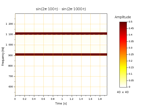
As a consequence of the sin(a).sin(b)=(cos(a-b)-cos(a+b))/2 formula,
both resulting frequencies [Fc-Fm, Fc+Fm] expected from the amplitude
modulation are clearly visible, with a shared amplitude=0.5
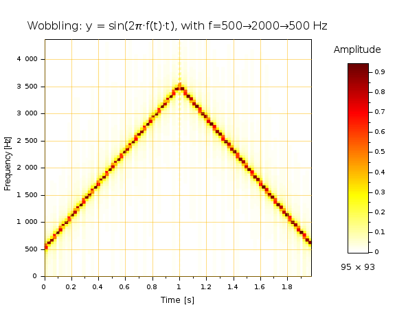
Example #3: Wobbling. Here, the frequency of a sine wave is linearly varied on [f0, f1]. This yields some actual higher frequencies, on [f0, 2*f1-f0]:
fs = 22050;
t = (0:fs-1)/fs;
f = 500*(1-t) + 2000*t;
y0 = sin(2*%pi*f.*t);
y = [y0 y0($:-1:1)];

playsnd(y/4)

clf
mapsound(y)
title "Wobbling: y = sin(2π⋅f(t)⋅t), with f=500→2000→500 Hz" fontsize 3.5
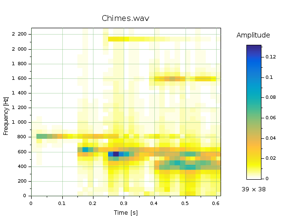
Example #4: Chimes.wav : a quite structured sound
[s1, fs1] = wavread('SCI/modules/sound/demos/chimes.wav');

playsnd([]), sleep(500), playsnd(s1/2), sleep(1000)

clf
mapsound(s1,, 2300, , parulacolormap)
title Chimes.wav fontsize 3.5
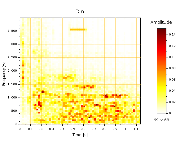
Example #5: Another sound, longer and more noisy
[s2, fs2] = wavread('SCI/modules/sound/tests/nonreg_tests/bug_467.wav');

playsnd([]), sleep(500), playsnd(s2/3)

clf
mapsound(s2, , 4000)
title Din fontsize 3.5
See also
History
| Version | Description |
| 6.1.1 | mapsound() rewritten: fmin and fmax merged into freqRange ; Colormap and data arguments added ; simpl removed. |
| Report an issue | ||
| << loadwave | Sons - fichiers audio | mu2lin >> |