plot2d

Arguments

x

a real matrix or vector. If omitted, it is assumed to be the vector 1:n where n is the number of curve points given by the y parameter.

y

a real matrix or vector.

<opt_args>

This represents a sequence of statements key1=value1,key2=value2,... where key1, key2,... can be one of the following:

logflag

sets the scale (linear or logarithmic) along the axes. The associated value should be a string with possible values: "nn", "nl" , "ln" and "ll" .

style

sets the style for each curve. The associated value should be a real vector with integer (positive or negative) values.

strf

controls the display of captions.

strf is a string of length 3 "xyz" (by default strf= "081" )

leg

sets the curves captions. The associated value should be a character string.

rect

sets the minimal bounds requested for the plot. The associated value should be a real vector with four entries: [xmin,ymin,xmax,ymax].

nax

sets the axes labels and tics definition. The associated value should be a real vector with four integer entries [nx,Nx,ny,Ny].

frameflag

controls the computation of the actual coordinate ranges from the minimal requested values. The associated value should be an integer ranging from 0 to 8.

axesflag

specifies how the axes are drawn. The associated value should be an integer ranging from 0 to 5 or 9 (default value).

Description

plot2d plots a set of 2D curves. If you are familiar with Matlab plot syntax, you should use plot.

If x and y are vectors, plot2d(x,y,<opt_args>) plots vector y versus vector x. x and y vectors should have the same number of entries.

If x is a vector and y a matrix plot2d(x,y,<opt_args>) plots each columns of y versus vector x. The number of rows of y must be equal to the number of x entries.

If x and y are matrices, plot2d(x,y,<opt_args>) plots each columns of y versus corresponding column of x. x and y must then have the same sizes.

If y is a vector, plot2d(y,<opt_args>) plots vector y versus vector 1:size(y,'*').

If y is a matrix, plot2d(y,<opt_args>) plots each columns of y versus vector 1:size(y,1).

The <opt_args> arguments should be used to customize the plot

logflag

This option may be used to set the scale (linear or logarithmic) along the axes. The associated value should be a string with possible values: "nn", "nl" , "ln" and "ll". "l" stands for logarithmic scale and graduations and "n" for normal scale.

style

This option may be used to specify how the curves are drawn. If this option is specified, the associated value should be a vector with as many entries as curves.

• if style(i) is strictly positive, the curve is drawn as plain line and style(i) defines the index of the color used to draw the curve (see getcolor). Note that the line style and the thickness can be set through the polyline entity properties (see polyline_properties).

  Piecewise linear interpolation is done between the given curve points.

• if style(i) is negative or zero, the given curve points are drawn using marks, abs(style(i)) defines the mark with id used. Note that the marks color and marks sizes can be set through the polyline entity properties (see polyline_properties).

strf

is a string of length 3 "xyz" (by default strf= "081")

x

controls the display of captions.

x=0

no caption.

x=1

captions are displayed. They are given by the optional argument leg.

y

controls the computation of the actual coordinate ranges from the minimal requested values. Actual ranges can be larger than minimal requirements.

y=0

no computation, the plot use the previous (or default) scale

y=1

from the rect arg

y=2

from the min/max of the x, y data

y=3

built for an isometric scale from the rect arg

y=4

built for an isometric plot from the min/max of the x, y data

y=5

enlarged for pretty axes from the rect arg

y=6

enlarged for pretty axes from the min/max of the x, y data

y=7

like y=1 but the previous plot(s) are redrawn to use the new scale

y=8

like y=2 but the previous plot(s) are redrawn to use the new scale

z

controls the display of information on the frame around the plot. If axes are requested, the number of tics can be specified by the nax optional argument.

z=0

nothing is drawn around the plot.

z=1

axes are drawn, the y=axis is displayed on the left.

z=2

the plot is surrounded by a box without tics.

z=3

axes are drawn, the y=axis is displayed on the right.

z=4

axes are drawn centred in the middle of the frame box.

z=5

axes are drawn so as to cross at point (0,0). If point (0,0) does not lie inside the frame, axes will not appear on the graph.

leg

This option may be used to sets the curve captions. It must be a string with the form "leg1@leg2@...." where leg1 , leg2 , etc. are respectively the captions of the first curve, of the second curve, etc. The default is " ".

The curve captions are drawn on below the x-axis. This option is not flexible enough, use the captions or legend functions preferably.

rect

This option may be used to set the minimal bounds requested for the plot. If this option is specified, the associated value should be a real vector with four entries:

[xmin,ymin,xmax,ymax]. xmin and xmax defines the bounds on the abscissae while ymin and ymax defines the bounds on the ordinates.

This argument may be used together with the frameflag option to specify how the axes boundaries are derived from the given rect argument. If the frameflag option is not given, it is supposed to be frameflag=7.

The axes boundaries can also be customized through the axes entity properties (see axes_properties).

nax

This option may be used to specify the axes labels and tics definition. The associated value should be a real vector with four integer entries [nx,Nx,ny,Ny].

Nx gives the number of main tics to be used on the x-axis (to use autoticks set it to -1), nx gives the number of subtics to be drawn between two main x-axis tics.

Ny and ny give similar information for the y-axis.

If axesflag option is not set nax option supposes that axesflag option has been set to 9.

frameflag

This option may be used to control the computation of the actual coordinate ranges from the minimal requested values. Actual ranges can be larger than minimal requirements.

frameflag=0

no computation, the plot use the previous (or default) scale.

frameflag=1

The actual range is the range given by the rect option.

frameflag=2

The actual range is computed from the min/max of the x and y data.

frameflag=3

The actual range is the range given by the rect option and enlarged to get an isometric scale.

frameflag=4

The actual range is computed from the min/max of the x and y data and enlarged to get an isometric scale.

frameflag=5

The actual range is the range given by the rect option and enlarged to get pretty axes labels.

frameflag=6

The actual range is computed from the min/max of the x and y data and enlarged to get pretty axes labels.

frameflag=7

like frameflag=1 but the previous plot(s) are redrawn to use the new scale. Used to add the current graph to a previous one.

frameflag=8

likeframeflag=2 but the previous plot(s) are redrawn to use the new scale. Used to add the current graph to a previous one.

frameflag=9

likeframeflag=8 but the range is enlarged to get pretty axes labels. This is the default value.

The axes boundaries can also be customized through the axes entity properties (see axes_properties)

axesflag

This option may be used to specify how the axes are drawn. The associated value should be an integer ranging from 0 to 5 :

axesflag=0

nothing is drawn around the plot (axes_visible=["off" "off"];box="off").

axesflag=1

axes are drawn, the y-axis is displayed on the left (axes_visible=["on" "on"];box="on",y_location="left").

axesflag=2

the plot is surrounded by a box without tics (axes_visible=["off" "off"];box="on").

axesflag=3

axes are drawn, the y-axis is displayed on the right (axes_visible=["on" "on"];box="off",y_location="right").

axesflag=4

axes are drawn centered in the middle of the frame, the box being not drawn (axes_visible=["on" "on"];box="off",x_location="middle", y_location="middle").

axesflag=5

axes are drawn centered in the middle of the frame similarly to axesflag=4, the difference being that the box is drawn (axes_visible=["on" "on"];box="on",x_location="middle",y_location="middle").

axesflag=9

axes are drawn, the y-axis is displayed on the left (axes_visible=["on" "on"];box="off",y_location="left"). This is the default value.

The axes aspect can also be customized through the axes entity properties (see axes_properties).

More information

By default, successive plots are superposed. To clear the previous plot, use clf() .

Enter the command plot2d() to see a demo.

Other high level plot2d functions exist:

• plot2d2 same as plot2d but the curve is supposed to be piecewise constant.

• plot2d3 same as plot2d but the curve is plotted with vertical bars.

• plot2d4 same as plot2d but the curve is plotted with vertical arrows.

Examples

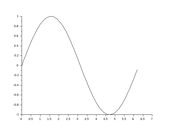
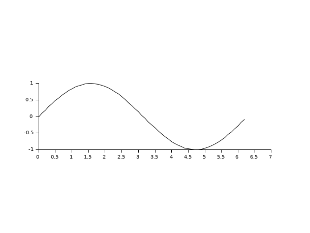
// x initialisation
x=[0:0.1:2*%pi]';
//simple plot
plot2d(sin(x));

clf();
x=[0:0.1:2*%pi]';
plot2d(x,sin(x));
//multiple plot

clf();
x=[0:0.1:2*%pi]';
plot2d(x,[sin(x) sin(2*x) sin(3*x)])

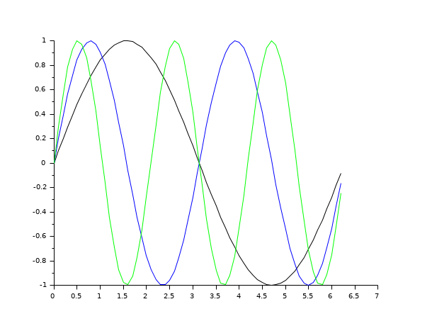
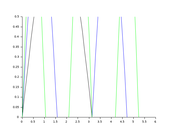
// multiple plot giving the dimensions of the frame
clf();
x=[0:0.1:2*%pi]';
plot2d(x,[sin(x) sin(2*x) sin(3*x)],rect=[0,0,6,0.5]);

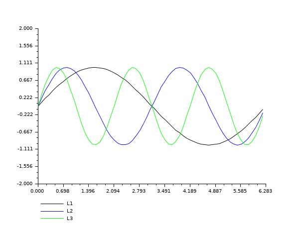
//multiple plot with captions and given tics + style
clf();
x=[0:0.1:2*%pi]';
plot2d(x,[sin(x) sin(2*x) sin(3*x)],..
       [1,2,3],leg="L1@L2@L3",nax=[2,10,2,10],rect=[0,-2,2*%pi,2]);

// isoview
clf();
x=[0:0.1:2*%pi]';
plot2d(x,sin(x),1,frameflag= 4);

// scale
clf();
x=[0:0.1:2*%pi]';
plot2d(x,sin(x),1,frameflag= 6);

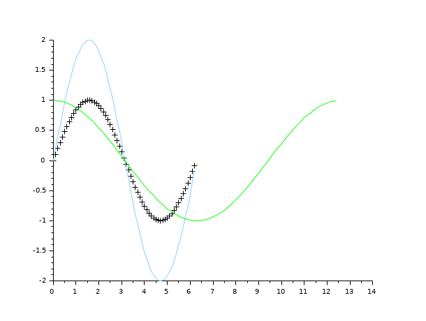
// auto scaling with previous plots + style
clf();
x=[0:0.1:2*%pi]';
plot2d(x,sin(x),-1);
plot2d(x,2*sin(x),12);
plot2d(2*x,cos(x),3);

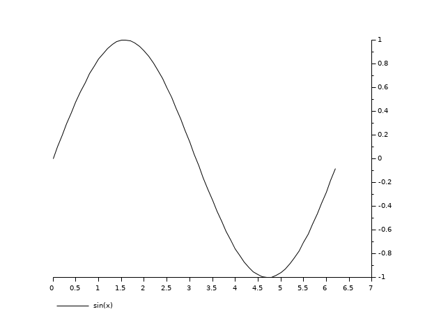
// axis on the right
clf();
x=[0:0.1:2*%pi]';
plot2d(x,sin(x),leg="sin(x)");
a=gca(); // Handle on axes entity
a.y_location ="right";

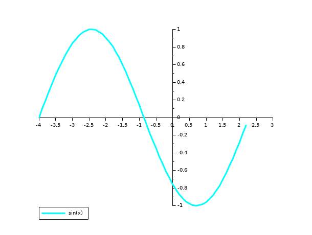
// axis centered at (0,0)
clf();
x=[0:0.1:2*%pi]';
plot2d(x-4,sin(x),1,leg="sin(x)");
a=gca(); // Handle on axes entity
a.x_location = "origin";
a.y_location = "origin";
// Some operations on entities created by plot2d ...
isoview
a=gca();
a.children // list the children of the axes.
// There are a compound made of two polylines and a legend
poly1= a.children(1).children(1); //store polyline handle into poly1
poly1.foreground = 4; // another way to change the style...
poly1.thickness = 3;  // ...and the thickness of a curve.
poly1.clip_state='off'; // clipping control
leg = a.children(2); // store legend handle into leg
leg.font_style = 9;
leg.line_mode = "on";
isoview off

See also

• plot — 2D plot
• plot2d2 — 2D plot (step function)
• plot2d3 — 2D plot (vertical bars)
• plot2d4 — 2D plot (arrows style)
• clf — Clears and resets a figure or a frame uicontrol
• xdel — supprime des fenêtres graphiques
• delete — delete a graphic entity and its children.