- Справка Scilab
- Signal Processing
- Filters
- How to design an elliptic filter
- analpf
- buttmag
- casc
- cheb1mag
- cheb2mag
- ell1mag
- eqfir
- eqiir
- faurre
- ffilt
- filt_sinc
- filter
- find_freq
- frmag
- fsfirlin
- group
- hilbert
- iir
- iirgroup
- iirlp
- kalm
- lev
- levin
- lindquist
- remez
- remezb
- srfaur
- srkf
- sskf
- syredi
- system
- trans
- wfir
- wfir_gui
- wiener
- wigner
- window
- yulewalk
- zpbutt
- zpch1
- zpch2
- zpell
Please note that the recommended version of Scilab is 2026.1.0. This page might be outdated.
See the recommended documentation of this function
How to design an elliptic filter
How to design an elliptic filter (analog and digital)
Description
The goal is to design a simple analog and digital elliptic filter.
Designing an analog elliptic filter
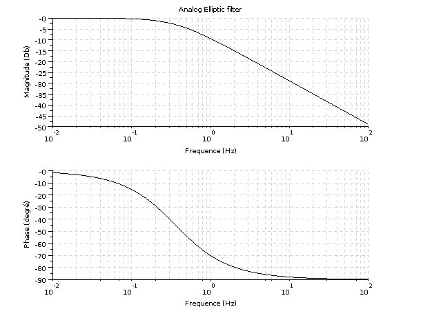
There are several possibilities to design an elliptic lowpass filter. We can use analpf or zpell. We will use zpell to produce the poles and zeros of the filter. Once we have got these poles and zeros, we will have to translate this representation into a syslin one.
And then, the filter can be represented in bode plot.
// analog elliptic (Bessel), order 2, cutoff 1 Hz
Epsilon = 3;  // ripple of filter in pass band (0<epsilon<1)
A       = 60; // attenuation of filter in stop band (A<1)
OmegaC  = 10; // pass band cut-off frequency in Hertz
OmegaR  = 50; // stop band cut-off frequency in Hertz

// Generate the filter
[_zeros,pols,gain] = zpell(3,60,10,50);

// Generate the equivalent linear system of the filter
num   = gain * real(poly(_zeros,'s'));;
den   = real(poly(pols,'s'));
elatf = syslin('c',num,den);

// Plot the resulting filter
bode(elatf,0.01,100);
title('Analog Elliptic filter');
Bode plot is only suited for analog filters.
If you want to design a highpass, bandpass or bandstop filter, you can first design a lowpass and then transform this lowpass filter using the trans function.
Designing a digital elliptic filter
Now, let's focus on how to produce a digital lowpass elliptic filter.
We can produce two kinds of digital filters:
an IIR (Infinite Impulse Response).
To compute such a filter, we can use the following functions:
a FIR (Finite Impulse Response).
To compute such a filter, we can use the following functions:
For our demonstration, we will use the iir function.
Order   = 2; // The order of the filter
Fs      = 1000; // The sampling frequency
Fcutoff = 40;   // The cutoff frequency

// We design a low pass elliptic filter
hz = iir(Order,'lp','ellip',[Fcutoff/Fs/2 0],[0.1 0.1]);

// We compute the frequency response of the filter
[frq,repf]=repfreq(hz,0:0.001:0.5);
[db_repf, phi_repf] = dbphi(repf);

// And plot the bode like representation of the digital filter
subplot(2,1,1);
plot2d(Fs*frq,db_repf);
xtitle('Obtained Frequency Response (Magnitude)');
subplot(2,1,2);
plot2d(Fs*frq,phi_repf);
xtitle('Obtained Frequency Response (Phase in degree)');
Here is the representation of the digital elliptic filter.
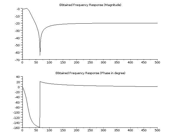
To represent the filter in phase and magnitude, we need first to convert the discrete impulse response into magnitude and phase using the dbphi function. This conversion is done using a set of normalized frequencies.
Filtering a signal using the digital filter
Designing a filter is a first step. Once done, this filter will be used to transform a signal. To get rid of some noise for example.
In the following examples, we will filter a gaussian noise.
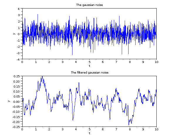
rand('normal');
Input = rand(1,1000); // Produce a random gaussian noise
t     = 1:1000;

sl= tf2ss(hz); // From transfert function to syslin representation
y = flts(Input,sl); // Filter the signal

subplot(2,1,1);
plot(t,Input);
xtitle('The gaussian noise','t','y');
subplot(2,1,2);
plot(t,y);
xtitle('The filtered gaussian noise','t','y');
Here is the representation of the signal before and after filtering.
As we can see in the result, the high frequencies of the noise have been removed and it remains only the low frequencies. The signal is still noisy, but it contains mainly low frequencies.
Filtering a signal using the analog filter
To filter a signal using an analog filter, we have two strategies:
transform the analog filter into a discrete one using the dscr function
apply the csim function to filter the signal
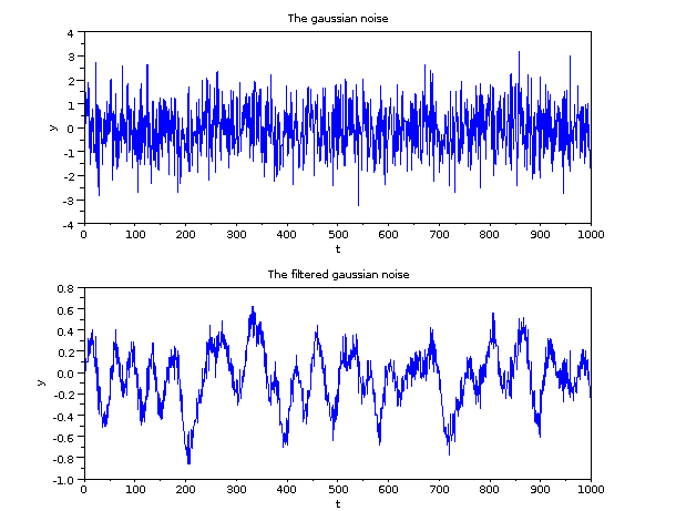
First, we try using the dscr + flts functions.
rand('normal');
Input = rand(1,1000); // Produce a random gaussian noise
n     = 1:1000; // The sample index

eldtf = dscr(elatf,1/100); // Discretization of the linear filter
y = flts(Input,eldtf); // Filter the signal

subplot(2,1,1);
plot(n,Input);
xtitle('The gaussian noise','n','y');
subplot(2,1,2);
plot(n,y);
xtitle('The filtered gaussian noise','n','y');
Here is the representation of the signal before and after filtering using the dscr + flts approach.
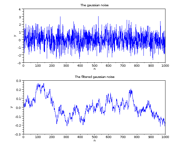
Next, we use the csim function.
rand('normal');
Input = rand(1,1000); // Produce a random gaussian noise
t     = 1:1000;
t     = t*0.01; // Convert sample index into time steps

y = csim(Input,t,elatf); // Filter the signal

subplot(2,1,1);
plot(t,Input);
xtitle('The gaussian noise','t','y');
subplot(2,1,2);
plot(t,y);
xtitle('The filtered gaussian noise','t','y');
Here is the representation of the signal before and after filtering using the csim approach.
The main difference between the dscr + flts approach and the csim approach: the dscr + flts uses samples whereas the csim functions uses time steps.
See also
- bode — Bode plot
- iir — iir digital filter
- poly — Определение полинома через указанные корни или коэффициенты или определение характеристического полинома квадратной матрицы.
- syslin — определение линейной системы
- zpell — lowpass elliptic filter
- flts — time response (discrete time, sampled system)
- tf2ss — transfer to state-space
- dscr — discretization of linear system
- csim — simulation (time response) of linear system
- trans — low-pass to other filter transform
- analpf — create analog low-pass filter
| Report an issue | ||
| << Filters | Filters | analpf >> |