- Справка Scilab
- Графики
- 2d_plot
- champ
- champ1
- champ properties
- comet
- contour2d
- contour2di
- contour2dm
- contourf
- errbar
- fchamp
- fec
- fec properties
- fgrayplot
- fplot2d
- grayplot
- grayplot properties
- graypolarplot
- histplot
- ВидЛинии
- Matplot
- Matplot1
- Matplot properties
- paramfplot2d
- plot
- plot2d
- plot2d2
- plot2d3
- plot2d4
- polarplot
- scatter
- Sfgrayplot
- Sgrayplot
Please note that the recommended version of Scilab is 2026.1.0. This page might be outdated.
See the recommended documentation of this function
plot
2D plot
Syntax
plot // demo
plot(y)
plot(x, y)
plot(x, fun)
plot(x, list(fun, param))
plot(.., LineSpec)
plot(.., LineSpec, GlobalProperty)
plot(x1, y1, LineSpec1, x2,y2,LineSpec2,...xN, yN, LineSpecN, GlobalProperty1,.. GlobalPropertyM)
plot(x1,fun1,LineSpec1, x2,y2,LineSpec2,...xN,funN,LineSpecN, GlobalProperty1, ..GlobalPropertyM)
plot(axes_handle,...)
Arguments
- x
vector or matrix of real numbers. If omitted, it is assumed to be the vector
1:nwherenis the number of curve points given by theyparameter.- y
vector or matrix of real numbers.
- fun, fun1, ..
handle of a function, as in
plot(x, sin).If the function to plot needs some parameters as input arguments, the function and its parameters can be specified through a list, as in
plot(x, list(delip, -0.4))- LineSpec
This optional argument must be a string that will be used as a shortcut to specify a way of drawing a line. We can have one
LineSpecperyor{x,y}previously entered.LineSpecoptions deals with LineStyle, Marker and Color specifiers (see LineSpec). Those specifiers determine the line style, mark style and color of the plotted lines.- GlobalProperty
This optional argument represents a sequence of couple statements
{PropertyName,PropertyValue}that defines global objects' properties applied to all the curves created by this plot. For a complete view of the available properties (see GlobalProperty).- axes_handle
This optional argument forces the plot to appear inside the selected axes given by
axes_handlerather than the current axes (see gca).
Description
plot plots a set of 2D curves. plot has been
rebuild to better handle Matlab syntax. To improve graphical
compatibility, Matlab users should use plot (rather than
plot2d).
Data entry specification :
In this paragraph and to be more clear, we won't mention
LineSpec nor GlobalProperty optional arguments
as they do not interfere with entry data (except for "Xdata",
"Ydata" and "Zdata" property, see
GlobalProperty). It is assumed that all those optional
arguments could be present too.
If y is a vector, plot(y) plots vector y
versus vector 1:size(y,'*').
If y is a matrix, plot(y) plots each columns of
y versus vector 1:size(y,1).
If x and y are vectors, plot(x,y) plots
vector y versus vector x. x and
y vectors should have the same number of entries.
If x is a vector and y a matrix plot(x,y)
plots each columns of y versus vector x. In this
case the number of columns of y should be equal to the number
of x entries.
If x and y are matrices, plot(x,y) plots each
columns of y versus corresponding column of x.
In this case the x and y sizes should be the
same.
Finally, if only x or y is a matrix, the
vector is plotted versus the rows or columns of the matrix. The choice is
made depending on whether the vector's row or column dimension matches the
matrix row or column dimension. In case of a square matrix (on
x or y only), priority is given to columns
rather than lines (see examples below).
 | When it is necessary and possible, plot transposes
x and y,
to get compatible dimensions; a warning is then issued. For instance,
when x has as many rows as y has columns.
If y is square, it is never transposed. |
y can also be a function defined as a macro or a
primitive. In this case, x data must be given (as a vector or
matrix) and the corresponding computation y(x) is done
implicitly.
The LineSpec and GlobalProperty arguments
should be used to customize the plot. Here is a complete list of the
available options.
- LineSpec
This option may be used to specify, in a short and easy manner, how the curves are drawn. It must always be a string containing references to LineStyle, Marker and Color specifiers.
These references must be set inside the string (order is not important) in an unambiguous way. For example, to specify a red long-dashed line with the diamond mark enabled, you can write :
'r--d'or'--dire'or'--reddiam'or another unambiguous statement... or to be totally complete'diamondred--'(see LineSpec).Note that the line style and color, marks color (and sizes) can also be (re-)set through the polyline entity properties (see polyline_properties).
- GlobalProperty
This option may be used to specify how all the curves are plotted using more option than via
LineSpec. It must always be a couple statement constituted of a string defining thePropertyName, and its associated valuePropertyValue(which can be a string or an integer or... as well depending on the type of thePropertyName). UsingGlobalProperty, you can set multiple properties : every properties available via LineSpec and more : the marker color (foreground and background), the visibility, clipping and thickness of the curves. (see GlobalProperty)Note that all these properties can be (re-)set through the polyline entity properties (see polyline_properties).
Remarks
By default, successive plots are superposed. To clear the previous
plot, use clf(). To enable auto_clear mode as
the default mode, edit your default axes doing:
da=gda();
da.auto_clear = 'on'
For a better display plot function may modify the box property of
its parent Axes. This happens when the parent Axes were created by the call to plot or were empty
before the call. If one of the axis is centered at origin,
the box is disabled.
Otherwise, the box is enabled.
For more information about box property and axis positioning see axes_properties
A default color table is used to color plotted curves if you do not specify a color. When drawing multiple lines, the plot command automatically cycles through this table. Here are the used colors:
R |
G |
B |
|---|---|---|
| 0. | 0. | 1. |
| 0. | 0.5 | 0. |
| 1. | 0. | 0. |
| 0. | 0.75 | 0.75 |
| 0.75 | 0. | 0.75 |
| 0.75 | 0.75 | 0. |
| 0.25 | 0.25 | 0.25 |
Enter the command plot to see a demo.
Examples
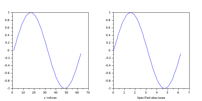
Simple plot of a single curve:
// Default abscissae = indices
subplot(1,2,1)
plot(sin(0:0.1:2*%pi))
xlabel("x indices")

// With explicit abscissae:
x = [0:0.1:2*%pi]';
subplot(1,2,2)
plot(x, sin(x))
xlabel("Specified abscissae")
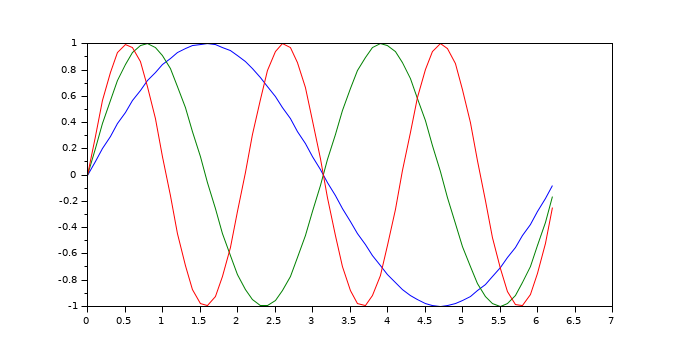
Multiple curves with shared abscissae: Y: 1 column = 1 curve:
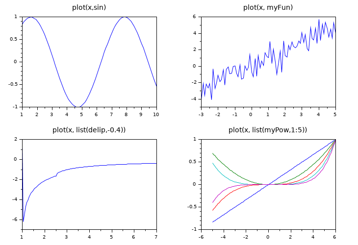
Specifying a macro or a builtin instead of explicit ordinates:
clf
subplot(2,2,1)         // sin() is a builtin
plot(1:0.1:10, sin)    // <=> plot(1:0.1:10, sin(1:0.1:10))
title("plot(x, sin)", "fontsize",3)

// with a macro:
deff('y = myFun(x)','y = x + rand(x)')
subplot(2,2,2)
plot(-3:0.1:5, myFun)
title("plot(x, myFun)", "fontsize",3)

// With functions with parameters:
subplot(2,2,3)
plot(1:0.05:7, list(delip, -0.4))  // <=> plot(1:0.05:7, delip(1:0.05:7,-0.4) )
title("plot(x, list(delip,-0.4))", "fontsize",3)

function Y=myPow(x, p)
    [X,P] = ndgrid(x,p);
    Y = X.^P;
    m = max(abs(Y),"r");
    for i = 1:size(Y,2)
        Y(:,i) = Y(:,i)/m(i);
    end
endfunction
x = -5:0.1:6;
subplot(2,2,4)
plot(x, list(myPow,1:5))
title("plot(x, list(myPow,1:5))", "fontsize",3)
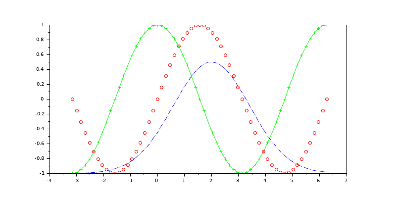
Setting curves simple styles when calling plot():
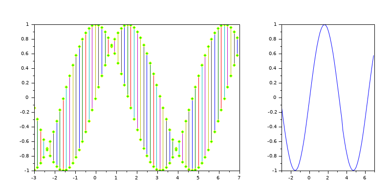
clf
t = -%pi:%pi/20:2*%pi;
// sin() : in Red, with O marks, without line
// cos() : in Green, with + marks, with a solid line
// gaussian: in Blue, without marks, with dotted line
gauss = 1.5*exp(-(t/2-1).^2)-1;

plot(t,sin,'ro', t,cos,'g+-', t,gauss,':b')
Vertical segments between two curves, with automatic colors, and using Global properties for markers styles. Targeting a defined axes.
clf
subplot(1,3,3)
ax3 = gca();         // We will draw here later
xsetech([0 0 0.7 1]) // Defines the first Axes area
t = -3:%pi/20:7;
// Tuning markers properties
plot([t ;t],[sin(t) ;cos(t)],'marker','d','markerFaceColor','green','markerEdgeColor','yel')

// Targeting a defined axes
plot(ax3, t, sin)
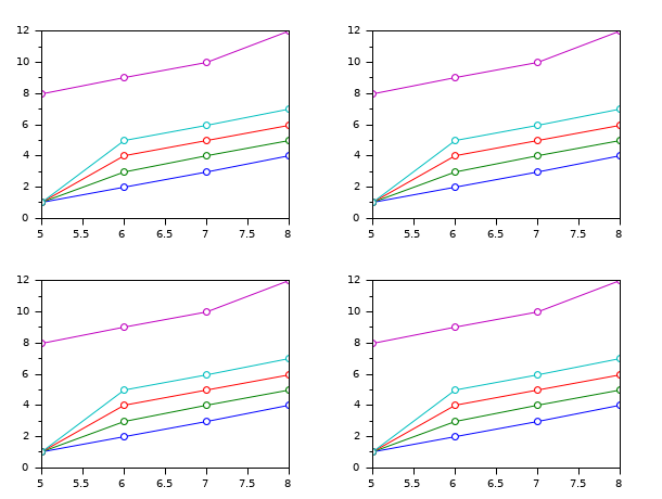
Case of a non-square Y matrix: When it is consistent and required, X or/and Y data are automatically transposed in order to become plottable.
clf()
x = [5 6 7 8]
y = [1   1   1   1   8
     2   3   4   5   9
     3   4   5   6  10
     4   5   6   7  12];

// Only one matching possibility case: how to make 4 identical plots in 4 manners...
// x is 1x4 (vector) and y is 4x5 (non square matrix)
subplot(221); plot(x', y , "o-");    // OK as is
subplot(222); plot(x , y , "o-");    // x is transposed
subplot(223); plot(x', y', "o-");    // y is transposed
subplot(224); plot(x , y', "o-");    // x and y are transposed
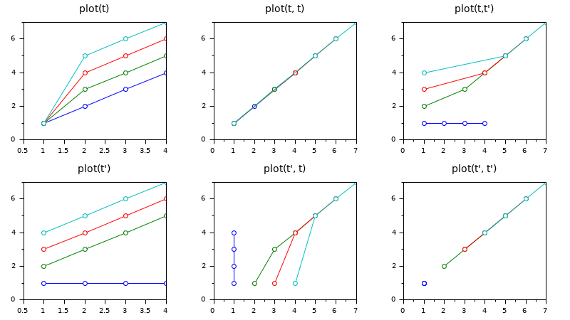
Case of a square Y matrix, and X implicit or square:
clf
t = [1   1   1   1
     2   3   4   5
     3   4   5   6
     4   5   6   7];

subplot(231), plot(t,"o-") , title("plot(t)",  "fontsize",3)
subplot(234), plot(t',"o-"), title("plot(t'')", "fontsize",3)

subplot(232), plot(t,t,"o-") , title("plot(t, t)",  "fontsize",3)
subplot(233), plot(t,t',"o-"), title("plot(t,t'')", "fontsize",3)

subplot(235), plot(t', t,"o-"),  title("plot(t'', t)",   "fontsize",3)
subplot(236), plot(t', t',"o-"), title("plot(t'', t'')", "fontsize",3)

for i=1:6, gcf().children(i).data_bounds([1 3]) = 0.5; end
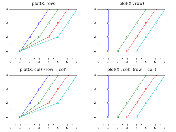
Special cases of a matrix X and a vector Y:
clf
X = [1   1   1   1
     2   3   4   5
     3   4   5   6
     4   5   6   7];
y = [1 2 3 4];

subplot(221), plot(X, y,  "o-"), title("plot(X, row)",  "fontsize",3)
        // equivalent to plot(t, [1 1 1 1; 2 2 2 2; 3 3 3 3; 4 4 4 4])
subplot(223), plot(X, y', "o-"), title("plot(X, col)  (row = col'')",  "fontsize",3)
subplot(222), plot(X',y,  "o-"), title("plot(X'', row)",  "fontsize",3)
subplot(224), plot(X',y', "o-"), title("plot(X'', col)  (row = col'')",  "fontsize",3)

for i = 1:4, gcf().children(i).data_bounds([1 3]) = 0.5; end
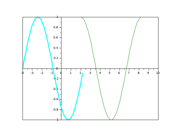
Post-tuning Axes and curves:
x=[0:0.1:2*%pi]';
plot(x-4,sin(x), x+2,cos(x))

// axis centered at (0,0)
a=gca(); // Handle on axes entity
a.x_location = "origin";
a.y_location = "origin";

// Some operations on entities created by plot ...
isoview on
a.children // list the children of the axes : here it is an Compound child composed of 2 entities
poly1= a.children.children(2); //store polyline handle into poly1
poly1.foreground = 4;  // another way to change the style...
poly1.thickness = 3;   // ...and the thickness of a curve.
poly1.clip_state='off' // clipping control
isoview off
See also
- plot2d — 2D plot
- plot2d2 — 2D plot (step function)
- plot2d3 — 2D plot (vertical bars)
- plot2d4 — 2D plot (arrows style)
- param3d — plots a single curve in a 3D cartesian frame
- surf — 3D surface plot
- scf — set the current graphic figure (window)
- clf — Clears and resets a figure or a frame uicontrol
- xdel — удаление графического окна
- delete — delete a graphic entity and its children.
- LineSpec — для быстрой настройки вида линий на графике
- Named colors — list of named colors
- GlobalProperty — для настройки вида объектов (кривых, поверхностей, ...) в командах plot или surf
History
| Версия | Описание |
| 6.0.1 | The "color"|"foreground", "markForeground", and "markBackground" GlobalProperty colors can now be chosen among the full predefined colors list, or by their "#RRGGBB" hexadecimal codes, or by their indices in the colormap. |
| 6.0.2 | Plotting a function fun(x, params) with input parameters is now possible with plot(x, list(fun, params)). |
| Report an issue | ||
| << paramfplot2d | 2d_plot | plot2d >> |