calfrq

Arguments

h

Linear system in state space or transfer representation ( see syslin )

fmin,fmax

real scalars (min and max frequencies in Hz)

frq

row vector (discretization of the frequency interval)

bnds

vector [Rmin Rmax Imin Imax] where Rmin and Rmax are the lower and upper bounds of the frequency response real part, Imin and Imax are the lower and upper bounds of the frequency response imaginary part,

split

vector of frq splitting points indexes

Description

frequency response discretization; frq is the discretization of [fmin,fmax] such that the peaks in the frequency response are well represented.

Singularities are located between frq(split(k)-1) and frq(split(k)) for k>1.

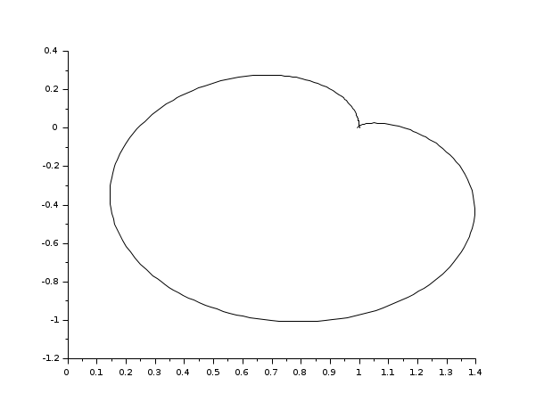
Examples

s=poly(0,'s')
h=syslin('c',(s^2+2*0.9*10*s+100)/(s^2+2*0.3*10.1*s+102.01))
h1=h*syslin('c',(s^2+2*0.1*15.1*s+228.01)/(s^2+2*0.9*15*s+225))
[f1,bnds,spl]=calfrq(h1,0.01,1000);
rf=repfreq(h1,f1);
plot2d(real(rf)',imag(rf)')

See also

• bode — Bode plot
• black — Black-Nichols diagram of a linear dynamical system
• nyquist — nyquist plot
• freq — frequency response
• repfreq — frequency response
• logspace — вектор с интервалами между элементами в логарифмическом масштабе