- Scilab Help
- Graphics
- 2d_plot
- LineSpec
- Matplot
- Matplot1
- Matplot properties
- Sfgrayplot
- Sgrayplot
- champ
- champ1
- champ properties
- comet
- contour2d
- contour2di
- contour2dm
- contourf
- errbar
- fchamp
- fec
- fec properties
- fgrayplot
- fplot2d
- grayplot
- grayplot properties
- graypolarplot
- histplot
- paramfplot2d
- plot
- plot2d
- plot2d2
- plot2d3
- plot2d4
- polarplot
- scatter
Please note that the recommended version of Scilab is 2026.1.0. This page might be outdated.
See the recommended documentation of this function
contourf
filled level curves of a surface on a 2D plot
Syntax
contourf(x, y, z, nz, [style, strf, leg, rect, nax])
Arguments
- x, y
two real row vectors of size
n1andn2: the grid.- z
a real matrix of size
(n1,n2), the values of the function.- nz
the level values or the number of levels.
- -
If
nzis an integer, its value gives the number of level curves equally spaced fromzmintozmaxas follows:z= zmin + (1:nz)*(zmax-zmin)/(nz+1)
 Note: that the
zminandzmaxlevels are not drawn (generically they are reduced to points) but they can be added with- -
If
nzis a vector,nz(i)gives the value of thei-th level curve.
- style, strf, leg, rect, nax
see
plot2d. The argumentstylegives the colors which are to be used for level curves. It must have the same size as the number of levels.
Description
contourf paints surface between two consecutive
level curves of a surface z=f(x,y) on a 2D plot.
The values of f(x,y) are given by the matrix
z at the grid points defined by
x and y.
You can change the format of the floating point number printed on
the levels by using xset("fpf",string) where
string gives the format in C format syntax (for
example string="%.3f"). Use string="" to
switch back to default format.
Enter the command contourf() to see a demo.
Examples
contourf(1:10,1:10,rand(10,10),5,1:5,"011"," ",[0,0,11,11])
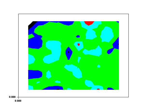
function z=peaks(x, y)
x1=x(:).*.ones(1,size(y,'*'));
y1=y(:)'.*.ones(size(x,'*'),1);
z =  (3*(1-x1).^2).*exp(-(x1.^2) - (y1+1).^2) ...
   - 10*(x1/5 - x1.^3 - y1.^5).*exp(-x1.^2-y1.^2) ...
   - 1/3*exp(-(x1+1).^2 - y1.^2)
endfunction

function z=peakit()
x=-4:0.1:4;y=x;z=peaks(x,y);
endfunction

z=peakit();

levels=[-6:-1,-logspace(-5,0,10),logspace(-5,0,10),1:8];
m=size(levels,'*');
n = fix(3/8*m);
r = [(1:n)'/n; ones(m-n,1)];
g = [zeros(n,1); (1:n)'/n; ones(m-2*n,1)];
b = [zeros(2*n,1); (1:m-2*n)'/(m-2*n)];
h = [r g b];
gcf().color_map = h;
xset('fpf',' ');
clf();
contourf([],[],z,[-6:-1,-logspace(-5,0,10),logspace(-5,0,10),1:8],0*ones(1,m))

xset('fpf','');
clf();
contourf([],[],z,[-6:-1,-logspace(-5,0,10),logspace(-5,0,10),1:8]);
See also
- contour — level curves on a 3D surface
- contour2d — level curves of a surface on a 2D plot
- contour2di — compute level curves of a surface on a 2D plot
- plot2d — 2D plot
| Report an issue | ||
| << contour2dm | 2d_plot | errbar >> |