Please note that the recommended version of Scilab is 2026.1.0. This page might be outdated.
However, this page did not exist in the previous stable version.
CVode
CVode (short for C-language Variable-coefficients ODE solver) is a numerical solver providing an efficient and stable method to solve Ordinary Differential Equations (ODEs) Initial Value Problems. It uses either BDF or Adams as implicit integration method, and Newton or Functional iterations
Description
Called by xcos, CVode (short for C-language Variable-coefficients ODE solver) is a numerical solver providing an efficient and stable method to solve Initial Value Problems of the form:

Starting with y0 , CVode approximates yn+1 with the formula:

with yn the approximation of y(tn) , and hn = tn - tn-1 the step size.
These implicit methods are characterized by their respective order q, which indicates the number of intermediate points required to compute yn+1 .
This is where the difference between BDF and Adams intervenes (Backward Differentiation Formula and Adams-Moulton formula):
 | If the problem is stiff, the user should select BDF: |
- q, the order of the method, is set between 1 and 5 (automated),
- K1 = q and K2 = 0.
In the case of nonstiffness, Adams is preferred:
- q is set between 1 and 12 (automated),
- K1 = 1 and K2 = q.
The coefficients are fixed, uniquely determined by the method type, its order, the history of the step sizes, and the normalization αn, 0 = -1 .
For either choice and at each step, injecting this integration in (1) yields the nonlinear system:

This system can be solved by either Functional or Newton iterations, described hereafter.
In both following cases, the initial "predicted" yn(0) is explicitly computed from the history data, by adding derivatives.
- Functional: this method only involves evaluations of f, it simply computes
yn(0)
by iterating the formula:


- Newton: here, we use an implemented direct dense solver on the linear system:

In both situations, CVode uses the history array to control the local error yn(m) - yn(0) and recomputes hn if that error is not satisfying.
The recommended choices are BDF / Newton for stiff problems and Adams / Functional for the nonstiff ones.
The function is called in between activations, because a discrete activation may change the system.
Following the criticality of the event (its effect on the continuous problem), we either relaunch the solver with different start and final times as if nothing happened, or, if the system has been modified, we need to "cold-restart" the problem by reinitializing it anew and relaunching the solver.
Averagely, CVode accepts tolerances up to 10-16. Beyond that, it returns a Too much accuracy requested error.
Examples
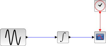
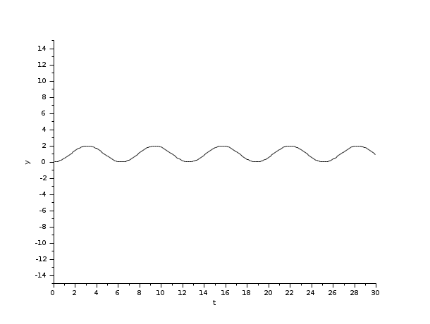
The integral block returns its continuous state, we can evaluate it with BDF / Newton by running the example:
// Import the diagram and set the ending time
loadScicos();
loadXcosLibs();
importXcosDiagram("SCI/modules/xcos/examples/solvers/ODE_Example.xcos");
scs_m.props.tf = 5000;

// Select the solver BDF / Newton
scs_m.props.tol(6) = 1;

// Start the timer, launch the simulation and display time
tic();
try xcos_simulate(scs_m, 4); catch disp(lasterror()); end
t = toc();
disp(t, "Time for BDF / Newton:");
The Scilab console displays:
Time for BDF / Newton:
 13.438
Now, in the following script, we compare the time difference between the methods by running the example with the four solvers in turn: Open the script
Results:
Time for BDF / Newton:
 18.894

Time for BDF / Functional:
 18.382

Time for Adams / Newton:
 10.368

Time for Adams / Functional:
 9.815
The results show that for a simple nonstiff continuous problem, Adams / Functional is fastest.
See Also
Bibliography
| Report an issue | ||
| << LSodar | Solvers | Runge-Kutta 4(5) >> |