Please note that the recommended version of Scilab is 2026.1.0. This page might be outdated.
See the recommended documentation of this function
Implicit Runge-Kutta 4(5)
Implicit Runge-Kutta is a numerical solver providing an efficient and stable implicit method to solve Ordinary Differential Equations (ODEs) Initial Value Problems. Called by xcos.
Description
Runge-Kutta is a numerical solver providing an efficient and stable fixed-size step method to solve Initial Value Problems of the form:

CVode and IDA use variable-size steps for the integration.
A drawback of that is the unpredictable computation time. With Runge-Kutta, we do not adapt to the complexity of the problem, but we guarantee a stable computation time.
This method being explicit, it can be used on stiff problems.
It is an enhancement of the backward Euler method, which approximates yn+1 by computing f(tn+h, yn+1) and truncating the Taylor expansion.
The implemented scheme is inspired from the "Low-Dispersion Low-Dissipation Implicit Runge-Kutta Scheme" (see bottom for link).
By convention, to use fixed-size steps, the program first computes a fitting h that approaches the simulation parameter max step size.
An important difference of implicit Runge-Kutta with the previous methods is that it computes up to the fourth derivative of y, while the others mainly use linear combinations of y and y'.
Here, the next value is determined by the present value yn plus the weighted average of three increments, where each increment is the product of the size of the interval, h, and an estimated slope specified by the function f(t,y). They are distributed approximately equally on the interval.
- k1 is the increment based on the slope near the quarter of the interval, using yn+ a11*h*k1, ,
- k2 is the increment based on the slope near the midpoint of the interval, using yn + a21*h*k1 + a22*h*k2, ,
- k3 is the increment based on the slope near the third quarter of the interval, using yn + a31*h*k1 + a32*h*k2 + a33*h*k3.
We see that the computation of ki requires ki, thus necessitating the use of a nonlinear solver (here, fixed-point iterations).
First, we set k0 = h * f(tn, yn) as first guess for all the ki, to get updated ki and a first value for yn+1 .
Next, we save and recompute yn+1 with those new ki.
Then, we compare the two yn+1 and recompute it until its difference with the last computed one is inferior to the simulation parameter reltol.
This process adds a significant computation time to the method, but greatly improves stability.
We can see that with the ki, we progress in the derivatives of yn . So in k3, we are approximating y(3)n , thus making an error in O(h4) . But choosing the right coefficients in the computation of the ki (notably the aij ) makes us gain an order, thus making a per-step total error in O(h5) .
So the total error is number of steps * O(h5) . And since number of steps = interval size / h by definition, the total error is in O(h4) .
That error analysis baptized the method implicit Runge-Kutta 4(5): O(h5) per step, O(h4) in total.
Although the solver works fine for max step size up to 10-3 , rounding errors sometimes come into play as we approach 4*10-4 . Indeed, the interval splitting cannot be done properly and we get capricious results.
Examples
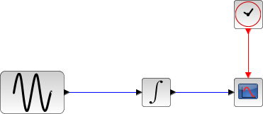
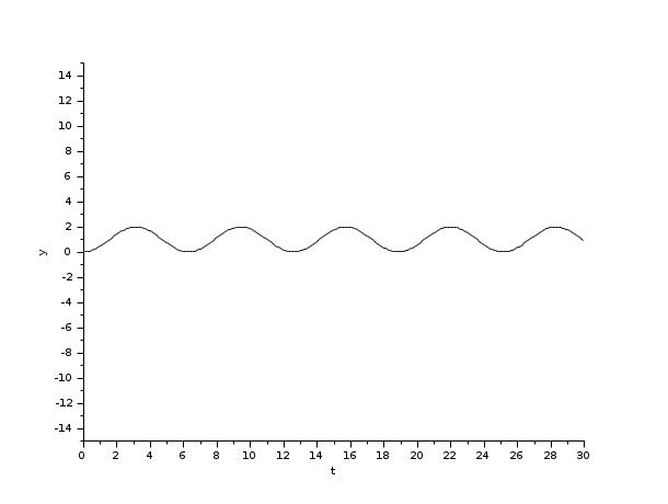
The integral block returns its continuous state, we can evaluate it with implicit RK by running the example:
// Import the diagram and set the ending time
loadScicos();
loadXcosLibs();
importXcosDiagram("SCI/modules/xcos/examples/solvers/ODE_Example.xcos");
scs_m.props.tf = 5000;

// Select the solver Runge-Kutta and set the precision
scs_m.props.tol(2) = 10^-10;
scs_m.props.tol(6) = 7;
scs_m.props.tol(7) = 10^-2;

// Start the timer, launch the simulation and display time
tic();
try xcos_simulate(scs_m, 4); catch disp(lasterror()); end
t = toc();
disp(t, "Time for implicit Runge-Kutta:");
The Scilab console displays:
Time for implicit Runge-Kutta:
 8.911
Now, in the following script, we compare the time difference between implicit RK and CVode by running the example with the five solvers in turn: Open the script
Time for BDF / Newton:
 18.894

Time for BDF / Functional:
 18.382

Time for Adams / Newton:
 10.368

Time for Adams / Functional:
 9.815

Time for implicit Runge-Kutta:
 6.652
These results show that on a nonstiff problem, for relatively same precision required and forcing the same step size, implicit Runge-Kutta competes with Adams / Functional.
Variable-size step ODE solvers are not appropriate for deterministic real-time applications because the computational overhead of taking a time step varies over the course of an application.
See Also
Bibliography
Journal of Computational Physics, Volume 233, January 2013, Pages 315-323 A low-dispersion and low-dissipation implicit Runge-Kutta scheme
History
| Версия | Описание |
| 5.4.1 | Implicit Runge-Kutta 4(5) solver added |
| Report an issue | ||
| << Dormand-Prince 4(5) | Solvers | IDA >> |