contour
level curves on a 3D surface
Syntax
contour(x, y, z, nz, [theta, alpha, leg, flag, ebox, zlev, fpf])
contour(x, y, z, nz, <opt_args>)
Arguments
- x,y
two real row vectors of size n1 and n2.
- z
real matrix of size (n1,n2), the values of the function or a Scilab function which defines the surface
z=f(x,y).- nz
the level values or the number of levels.
- -
If
nzis an integer, its value gives the number of level curves equally spaced from zmin to zmax as follows:z= zmin + (1:nz)*(zmax-zmin)/(nz+1)
 Note that the
zminandzmaxlevels are not drawn (generically they are reduced to points) but they can be added with- -
If
nzis a vector,nz(i)gives the value of the ith level curve. Note that it can be useful in order to seezminandzmaxlevel curves to add an epsilon tolerance:nz=[zmin+%eps,..,zmax-%eps].
- <opt_args>
a sequence of statements
key1=value1, key2=value2, ... where keys may betheta,alpha,leg,flag,ebox,zlev(see below). In this case, the order has no special meaning.- theta, alpha
real values giving in degree the spherical coordinates of the observation point.
- leg
string defining the captions for each axis with @ as a field separator, for example "X@Y@Z".
- flag
a real vector of size three
flag=[mode,type,box].- mode
string representation mode.
- mode=0:
the level curves are drawn on the surface defined by (x,y,z).
- mode=1:
the level curves are drawn on a 3D plot and on the plan defined by the equation z=zlev.
- mode=2:
the level curves are drawn on a 2D plot.
- type
an integer (scaling).
- type=0
the plot is made using the current 3D scaling (set by a previous call to
param3d,plot3d,contourorplot3d1).- type=1
rescales automatically 3d boxes with extreme aspect ratios, the boundaries are specified by the value of the optional argument
ebox.- type=2
rescales automatically 3d boxes with extreme aspect ratios, the boundaries are computed using the given data.
- type=3
3d isometric with box bounds given by optional
ebox, similarly totype=1- type=4
3d isometric bounds derived from the data, similarly to
type=2- type=5
3d expanded isometric bounds with box bounds given by optional
ebox, similarly totype=1- type=6
3d expanded isometric bounds derived from the data, similarly to
type=2
- box
an integer (frame around the plot).
- box=0
nothing is drawn around the plot.
- box=1
unimplemented (like box=0).
- box=2
only the axes behind the surface are drawn.
- box=3
a box surrounding the surface is drawn and captions are added.
- box=4
a box surrounding the surface is drawn, captions and axes are added.
- ebox
used when
typeinflagis 1. It specifies the boundaries of the plot as the vector[xmin,xmax,ymin,ymax,zmin,zmax].- zlev
real number.
- fpf
You can change the format of the floating point number printed on the levels where
fpfis the format in C format syntax (for examplefpf="%.3f"). Setfpfto " " implies that the level are not drawn on the level curves. If not given, the default format is"%.2g".
Description
contour draws level curves of a surface z=f(x,y). The level curves are
drawn on a 3D surface. The optional arguments are the same as for the function
plot3d (except zlev) and their meanings are the same.
They control the drawing of level curves on a 3D plot.
Only flag(1)=mode has a special meaning.
- mode=0
the level curves are drawn on the surface defined by (x,y,z).
- mode=1
the level curves are drawn on a 3D plot and on the plan defined by the equation z=zlev.
- mode=2
the level curves are drawn on a 2D plot.
Usually we use contour2d to draw levels curves on a 2D plot.
Enter the command contour() to see a demo.
Examples
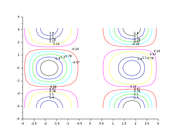
t=linspace(-%pi,%pi,30);
function z=my_surface(x, y),z=x*sin(x)^2*cos(y),endfunction
contour(t,t,my_surface,10)
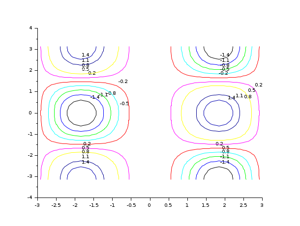
t=linspace(-%pi,%pi,30);
clf()
function z=my_surface(x, y),z=x*sin(x)^2*cos(y),endfunction
// changing the format of the printing of the levels
contour(t,t,my_surface,10, fpf="%.1f")
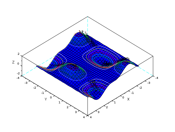
// 3D
t=linspace(-%pi,%pi,30);
function z=my_surface(x, y),z=x*sin(x)^2*cos(y),endfunction
z=feval(t,t,my_surface);
plot3d(t,t,z);contour(t,t,z+0.2*abs(z),20,flag=[0 2 4]);
| Report an issue | ||
| << comet3d | 3d_plot | eval3dp >> |