interp1
1D interpolation in nearest, linear or spline mode
Syntax
yp = interp1(y, xp)
yp = interp1(x, y, xp)
yp = interp1(.., xp, method)
yp = interp1(.., xp, method, extrapolation)
Arguments
- x
- vector of at least 2 real numbers: Abscissas of known interpolation nodes,
without duplicates. By default,
- if
yis a vector:x=1:length(y). - if
yis a matrix or an hypermatrix:x=1:size(y,1).
- if
- y
- vector, matrix or hypermatrix of real or complex numbers: values at known
interpolation nodes, at the corresponding
xabscissas.- if
yis a vector,xandymust have the same length. - if
yis a matrix or an hypermatrix, we must havelength(x)==size(y,1). Each column ofyis then interpolated versus the samexabscissas, for the givenxp.
- if
- xp
- scalar, vector, matrix or hypermatrix or decimal numbers: abscissas of
points whose values
ypmust be computed according to data of interpolation nodes. - yp
- vector, matrix, or hypermatrix of numbers: interpolated
yvalues at the givenxp.- if
yis a vector:yphas the size ofxp. - if
yis a matrix or an hypermatrix:- if
xpis a scalar or a vector:size(yp)is[length(xp) size(y)(2:$)] - if
xpis a matrix or an hypermatrix:size(yp)is[size(xp) size(y)(2:$)]
- if
- if
- method
- string defining the interpolation method. Possible values and processing are:
"linear": linear interpolation between consecutive nodes, used by default. "spline": interpolation by cubic splines "nearest": for each value xp(j), yp(j) takes the value or y(i) corresponding to x(i) the nearest neighbor of xp(j)
- extrapolation
- string or number defining the yp(j) components for xp(j) values outside the
[x(1)=min(x),x($)=max(x)] interval. We suppose here-below that
xandyhave already been sorted accordingly."extrap": interp1(x,y,xp, method, "extrap")is equivalent tointerp1(x,y,xp, method, method)."linear": Can be used with the "spline"(and obviously"linear") interpolation methods."periodic": This extrapolation type can be used with the "linear"or"spline"interpolation methods. Then: ifyis a vector,y(1)==y($)is required ; otherwisey(1,:)==y($,:)is required."edgevalue": Then yp(i)=y(1)for everyxp(i)<x(1), andyp(i)=y($)for everyxp(i)>x($).padding: paddingis a decimal or complex number used to setyp(i)=paddingfor everyxp(i) ∉ [min(x),max(x)]. Example:yi=interp1(x,y,xp,method, 0).(none): By default, the extrapolation is performed by splines when splines are used for the interpolation, and by padding with %nan when the interpolation is linear or by "nearest" node.
Description
Given (x,y,xp), this function computes the yp
components corresponding to xp by the interpolation between known
data provided by (x,y) nodes.
x is priorly sorted in ascending order, and
y values or per column are then sorted accordingly.
Interpolation of complex values: When
y is complex, its real and imaginary parts are interpolated
separately, and then added to build the complex yp.
interp1(x,y,xp,"nearest"): For any xp
at the middle of an [x(i),x(i+1)] interval, the upper
bound x(i+1) is considered as the nearest
x value, and yp=y(i+1) is assigned.
linear interpolations
They are performed through thelinear_interpn(..) function,
with the corresponding "edgevalue"→"C0",
"linear"→"natural", "periodic"→"periodic"
extrapolation option.spline interpolations
interp1(..,xp,"spline") or
interp1(..,xp,"spline","spline") or
interp1(..,xp,"spline","extrap")
use not_a_knot edges conditions. Extrapolation is performed
by using both spline polynomials computed at the (x,y) edges.
interp1(..,xp,"spline","edgevalue")
uses not_a_knot edges conditions and then calls
interp(..,"C0") to perform the actual interpolation
and extrapolation.
interp1(..,xp,"spline","periodic")
calls both splin(..) and then interp(..)
with their "periodic" option.
interp1(..,xp,"spline","linear")
calls splin(..,"natural") for linear edges conditions,
and then feeds interp(..,"linear").
Examples
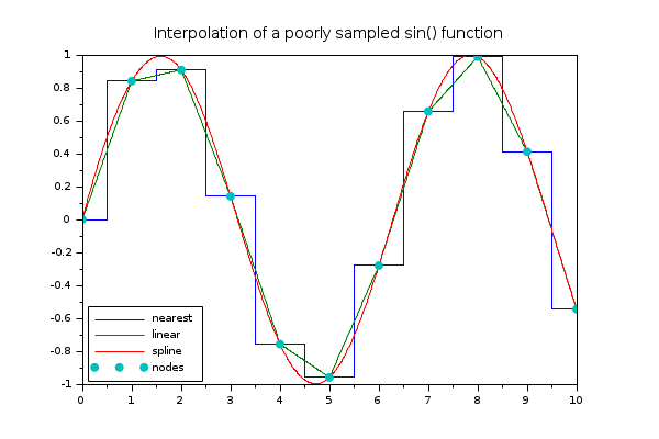
x = linspace(0, 10, 11)';
y = sin(x);
xx = linspace(0,10,1000)';
yy2 = interp1(x, y, xx, 'linear');
yy1 = interp1(x, y, xx, 'nearest');
yy3 = interp1(x, y, xx, 'spline');
clf
h = plot(xx, [yy1 yy2 yy3], x, y, '.')
h(1).mark_size = 8;
title "Interpolation of a poorly sampled sin() function" fontsize 3
legend(['nearest','linear','spline','nodes'], "in_lower_left");
See also
- interp — função de avaliação de spline cúbico
- splin — interpolação por spline cúbico
- linear_interpn — interpolação linear n-dimensional
History
| Version | Description |
| 6.1.1 |
|
| Report an issue | ||
| << interp | Interpolação | interp2d >> |