- Ajuda do Scilab
- Biblioteca de Gráficos
- 2d_plot
- champ
- champ1
- champ_properties
- comet
- contour2d
- contour2di
- contour2dm
- contourf
- cutaxes
- errbar
- fchamp
- fec
- fec properties
- fgrayplot
- fplot2d
- grayplot
- grayplot_properties
- graypolarplot
- histplot
- LineSpec
- loglog
- Matplot
- Matplot1
- Matplot properties
- paramfplot2d
- plot
- plot2d
- plot2d2
- plot2d3
- plot2d4
- plotimplicit
- polarplot
- scatter
- semilogx
- semilogy
- Sfgrayplot
- Sgrayplot
Please note that the recommended version of Scilab is 2026.0.1. This page might be outdated.
See the recommended documentation of this function
comet
2D comet animated plot
Syntax
comet(y)
comet(x, y)
comet(x, y, Lf)
comet(x, fun)
comet(x, fun, Lf)
comet(..., "colors",c)
Parameters
- x
- a real vector or matrix. If omitted, it is assumed to be the vector
1:npwherenpis the total number of curve points (see below). As a matrix, each column defines the abscissae of the trace of a separate comet. - y
- a real vector or matrix. As a matrix, each column defines the ordinates
of the trace of a separate comet.
nc=size(y,"c")is the number of comets simultaneously drawn. - Lf
- a real scalar in the interval
[0,1[. Default value is 0.1: It defines the Leading fraction of the comet's trace. Thek=Lf*npmost recent points are plotted in thicker line. - fun
- a scilab function with syntax
y = fun(x).funcan also be a polynomial or a rational fraction. - c
nccolors of thenccomets traces. They may be specified as a vector ofnccolor indices or color names or "#RRGGBB" hexadecimal color codes. Or by a matrix (ncx3) of[r,g,b]vectors of Red-Green-Blue intensities in the [0,1] interval.
Description
If (x,y) are two vectors, this function draws a 2D comet animated
plot showing the progression of the curve (x(1:m),y(1:m)) for
m varying from 1 to
np=length(x).
The plot is made of three parts:
| a head | mark that shows the current (x(i),y(i)) position. |
| a body | consisting in the k=round(Lf*np) most recent points
of the trajectory, displayed as a thicker part of the trace. |
| a tail | that shows the (x(1:i-k),y(1:i-k)) part of the curve. |
comet(x,fun,...) is equivalent to
comet(x, feval(x,fun),...).
If x and y are matrices with identical sizes,
then animated curves are drawn for each pair (x(:,j),y(:,j)).
In this case np is the number of rows of
x and y.
comet(...,"colors",c) can be used to set the colors of each
trajectory.
Examples
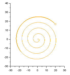
// One comet in spiral:
t = linspace(0, 10*%pi, 500);
clf, isoview
comet(t.*sin(t), t.*cos(t), "colors", "orange")

// Two simultaneous comets with default colors:
t = linspace(0, 10*%pi, 500)';
clf
comet(t.*sin(t), [t.*sin(2*t) t.*sin(3*t)])
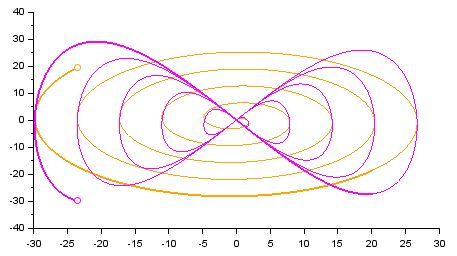
// Chosen colors:
t = linspace(0, 10*%pi, 500)';
clf
comet(t.*sin(t), [t.*cos(t) t.*sin(2*t)], "colors", ["orange" "mag"])

See also
- comet3d — 3D comet animated plot
- paramfplot2d — Esboço animado 2d, curva definida por uma função
- realtime — sets the time unit
- colors names — Lista dos nomes das cores
History
| Versão | Descrição |
| 5.3.2 | Function comet() introduced. |
| 6.1.0 | Colors can now be specified also by their name, or by their "#RRGGBB" hexadecimal code, or by their [r g b] Red-Green-Blue intensities. |
| Report an issue | ||
| << champ_properties | 2d_plot | contour2d >> |