Please note that the recommended version of Scilab is 2026.0.1. This page might be outdated.
See the recommended documentation of this function
ndgrid
build matrices or N-D arrays by replicating some template vectors
Syntax
[X, Y] = ndgrid(x)
[X, Y] = ndgrid(x,y)
[X, Y, Z] = ndgrid(x,y,z)
[X, Y, Z, T] = ndgrid(x,y,z,t)
[X1, X2, ..., Xm] = ndgrid(x1,x2,...,xm)
Arguments
- x, y, z, ...
vectors of any data types. They may have distinct data types. By default,
y=x.- X, Y, Z, ...
matrices in case of 2 input arguments, or hypermatrices otherwise. They all have the same sizes:
size(x,"*")rows,size(y,"*")columns,size(z,"*")layers, etc. They have the datatypes of respective input vectors:typeof(X)==typeof(x),typeof(Y)==typeof(y), etc.
Description
The first application of ndgrid is to build a grid of nodes meshing the 2D or 3D or N-D space according to 2, 3, or more sets x, y, etc.. of "template" coordinates sampled along each direction/dimension of the space that you want to mesh.
Hence, the matrix or hypermatrix X is made by replicating the vector x as all its columns ; the matrix or hypermatrix Y is made by replicating the vector y as all its rows ; Z is made of replicating the vector z along all its local thicknesses (3rd dimension); etc.
--> [X, Y] = ndgrid([1 3 4], [0 2 4 6])
 X  =
   1.   1.   1.   1.
   3.   3.   3.   3.
   4.   4.   4.   4.

 Y  =
   0.   2.   4.   6.
   0.   2.   4.   6.
   0.   2.   4.   6.
Then, the coordinates of the node(i,j) in the 2D space will be simply [x(i), y(j)] now given by [X(i,j), Y(i,j)]. As well, the coordinates of a node(i,j,k) of a 3D grid will be [x(i), y(j), z(k)] now given by [X(i,j,k), Y(i,j,k), Z(i,j,k)].
This replication scheme can be generalized to any number of dimensions, as well to any type of uniform data. Let's for instance consider 2 attributes:
- The first is a number, to be chosen from the vector say
n= [ 3 7 ] - The second is a letter, to be chosen from the vector say
c= ["a" "e" "i" "o" "u" "y"]
--> [N, C] = ndgrid([3 7],["a" "e" "i" "o" "u" "y"])
 C  =
!a  e  i  o  u  y  !
!a  e  i  o  u  y  !

 N  =
   3.   3.   3.   3.   3.   3.
   7.   7.   7.   7.   7.   7.
Then, the object(i,j) will have the properties {n(i) c(j)} that now can be addressed with {N(i,j) C(i,j)}. This kind of grid may be useful to initialize an array of structures.
Following examples show how to use X, Y, Z in most frequent applications.
Examples
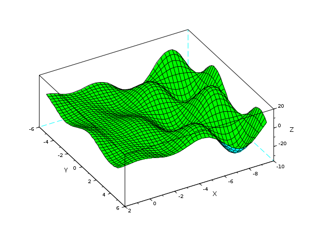
Example #1:
// Create a simple 2d grid
x = linspace(-10,2,40);
y = linspace(-5,5,40);
[X,Y] = ndgrid(x,y);

// Compute ordinates Z(X,Y) on the {X, Y} grid and plot Z(X,Y)
Z = X - 3*X.*sin(X).*cos(Y-4) ;

clf()
plot3d(x,y,Z, flag=[color("green") 2 4], alpha=7, theta=60); show_window()

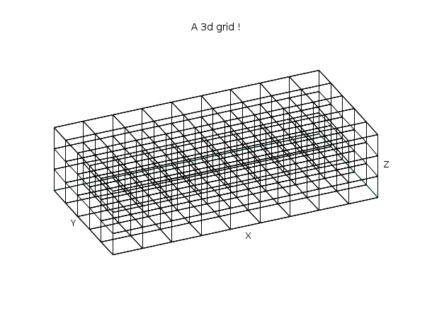
Example #2:
// Create a simple 3d grid
nx = 10; ny = 6; nz = 4;
x = linspace(0,2,nx);
y = linspace(0,1,ny);
z = linspace(0,0.5,nz);
[X,Y,Z] = ndgrid(x,y,z);

// Try to display this 3d grid
XF=[]; YF=[]; ZF=[];

for k=1:nz
   [xf,yf,zf] = nf3d(X(:,:,k),Y(:,:,k),Z(:,:,k));
   XF = [XF xf]; YF = [YF yf]; ZF = [ZF zf];
end

for j=1:ny
   [xf,yf,zf] = nf3d(matrix(X(:,j,:),[nx,nz]),...
                     matrix(Y(:,j,:),[nx,nz]),...
                     matrix(Z(:,j,:),[nx,nz]));
   XF = [XF xf]; YF = [YF yf]; ZF = [ZF zf];
end

clf()
plot3d(XF,YF,ZF, flag=[0 6 3], 66, 61,leg="X@Y@Z")
xtitle("A 3d grid !"); show_window()

Example #3: Creates a table of digrams:
[c1, c2] = ndgrid(["a" "b" "c"], ["a" "b" "c" "d" "e" "f" "g" "h"])
c1+c2
--> [c1, c2] = ndgrid(["a" "b" "c"], ["a" "b" "c" "d" "e" "f" "g" "h"])
 c2  =
!a  b  c  d  e  f  g  h  !
!a  b  c  d  e  f  g  h  !
!a  b  c  d  e  f  g  h  !

 c1  =
!a  a  a  a  a  a  a  a  !
!b  b  b  b  b  b  b  b  !
!c  c  c  c  c  c  c  c  !

--> c1+c2
 ans  =
!aa  ab  ac  ad  ae  af  ag  ah  !
!ba  bb  bc  bd  be  bf  bg  bh  !
!ca  cb  cc  cd  ce  cf  cg  ch  !
See also
History
| バージョン | 記述 |
| 6.0.0 | Extension to all homogeneous datatypes ([], booleans, encoded integers, polynomials, rationals, strings). Revision of the help page. |
| 6.0.1 | ndgrid(x) is now accepted: Default y=x. |
| Report an issue | ||
| << meshgrid | elementarymatrices | ones >> |