Please note that the recommended version of Scilab is 2026.1.0. This page might be outdated.
See the recommended documentation of this function
sgrid
draws a s-plane grid
Syntax
sgrid()
sgrid(zeta, wn)
sgrid(.., colors)
sgrid(.., "new")
Arguments
- zeta
vector of damping factors. Only values in
[0 1]are taken into account. The default values are ~ cosd(90:-10:0) =[0 0.17 0.34 0.5 0.64 0.77 0.87 0.94 0.985 1].- wn
array of natural frequencies in Hz. only positive values are taken into account. If not given it is computed by the program to fit with the boundaries of the plot.
- colors
a scalar or a vector with 2 elements [circles_col, rays_col], specifying the color(s) of circles and rays of the frame, and their labels: predefined colors names (like "red"), or colors hexadecimal codes (like "#34DDFA"), or colors indices in the current colormap are accepted.
- "new"
This option clears all contents of the current axes before plotting the grid. It may be specified at any position among input arguments.
Description
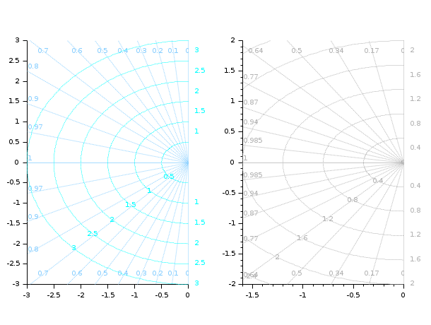
The sgrid function is often used to draw a grid
for Evans root locus of continuous time linear systems. In such a
case the sgrid function should be called after
the call to evans. For discrete time linear
systems one should use zgrid function instead.
sgrid plots curves of constant damping ratio at values given
by zeta, and constant natural frequency at values given by
wn.
The colors argument may be used to assign a color for constant
damping ratio curves (colors(2)) and for constant natural
frequency curves (colors(1)).
sgrid(), sgrid("new"), sgrid(colors) or
sgrid(colors, "new") plots a default grid.
Examples
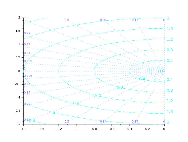
Post-tuning graphical elements of the grid:
sgrid()

sGrid = gca().children.children.children;
i = find(sGrid(3:$).type=="Polyline" & sGrid(1:$-2).type=="Polyline",1);

Circles = sGrid(1:i-1);
Circ_text = Circles(Circles.type=="Text");      // Labels
Circ_text.font_size = 2;
Circ_lines = Circles(Circles.type=="Polyline"); // Circles
Circ_lines.line_style = 8;

Rays = sGrid(i:$);
Rays(Rays.type=="Text").font_foreground = color("light slate blue");
Rays_lines = Rays(Rays.type=="Polyline");
set(Rays_lines, "line_style", 9, "thickness", 1.5);
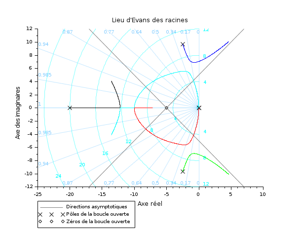
Evans plot + a s grid:
See also
- evans — Evans root locus
- zgrid — zgrid plot
- hallchart — Draws a Hall chart
- nicholschart — Nichols chart
History
| Version | Description |
| 6.0.2 | colors can be specified by their names or by their #RRGGBB code |
| Report an issue | ||
| << routh_t | Stabilité | show_margins >> |