- Aide de Scilab
- Graphiques
- 2d_plot
- champ
- champ1
- champ properties
- comet
- contour2d
- contour2di
- contour2dm
- contourf
- cutaxes
- errbar
- fchamp
- fec
- fec properties
- fgrayplot
- fplot2d
- grayplot
- grayplot properties
- graypolarplot
- histplot
- LineSpec
- loglog
- Matplot
- Matplot1
- Matplot properties
- paramfplot2d
- plot
- plot2d
- plot2d2
- plot2d3
- plot2d4
- plotimplicit
- polarplot
- scatter
- semilogx
- semilogy
- Sfgrayplot
- Sgrayplot
Please note that the recommended version of Scilab is 2026.1.0. This page might be outdated.
See the recommended documentation of this function
plotimplicit
Plots the (x,y) lines solving an implicit equation or Function(x,y)=0
Syntax
plotimplicit(fun)
plotimplicit(fun, x_grid)
plotimplicit(fun, x_grid, y_grid)
plotimplicit(fun, x_grid, y_grid, plotOptions)
Arguments
- fun
It may be one of the following:
- A single Scilab-executable string expression of literal scalar
variables "x" and "y" representing two scalar real numbers.
Examples:
"x^3 + 3*y^2 = 1/(2+x*y)","(x-y)*(sin(x)-sin(y))"(implicitly = 0). - The identifier of an existing function of two variables x and y.
Example:
besselj(not"besselj"). - A list, gathering a Scilab or built-in function identifier,
followed by the series of its parameters.
Example: After
function r = test(x,y,a), r = x.*(y-a), endfunction,funcan belist(test, 3.5)to consider and computetest(x, y, 3.5).
- A single Scilab-executable string expression of literal scalar
variables "x" and "y" representing two scalar real numbers.
Examples:
- x_grid, y_grid
x_gridandy_griddefine the cartesian grid of nodes wherefun(x,y) must be computed.By default,
x_grid = [-1,1]andy_grid = x_gridare used. To use default values, just specify nothing. Example skippingy_grid:plotimplicit(fun, x_grid, , plotOptions).Explicit
x_gridandy_gridvalues can be specified as follow:- A vector of 2 real numbers = bounds of the x or y domain. Example:
[-2, 3.5]. Then the given interval is sampled with 201 points. - A vector of more than 2 real numbers = values where the function
is computed. Example:
-1:0.1:2. - The colon
:. Then the considered interval is given by the data bounds of the current or default axes. This allows to overplot solutions of multiple equations on a shared (x,y) domain, with as many call toplotimplicit(..)as required.
 The bounds of the 1st plot drawn by
plotimplicit(..)are set according to the bounds of the solutions offun. Most often they are (much) narrower thanx_gridandy_gridbounds.- A vector of 2 real numbers = bounds of the x or y domain. Example:
- plotOptions
- List of plot() line-styling options used when plotting the solutions curves.
Description
plotimplicit(fun, x_grid, y_grid) evaluates fun
on the nodes (x_grid, y_grid), and then
draws the (x,y) contours solving the equation fun or such that
fun(x,y) = 0.
When no root curve exists on the considered grid, plotimplicit
yields a warning and plots an empty axes.
 |
|
Examples
With the literal expression of the cartesian equation to plot:
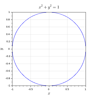
// Draw a circle of radius 1 according to its cartesian equation:
plotimplicit "x^2 + y^2 = 1"

xgrid(color("grey"),1,7)
isoview
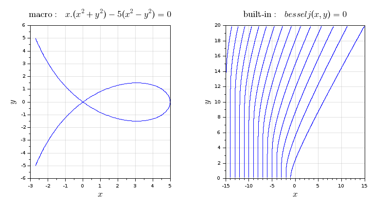
With the identifier of the function whose root lines must be plotted:
clf
// 1) With a function in Scilab language (macro)
function z=F(x, y)
    z = x.*(x.^2 + y.^2) - 5*(x.^2 - y.^2);
endfunction

// Draw the curve in the [-3 6] x [-5 5] range
subplot(1,2,1)
plotimplicit(F, -3:0.1:6, -5:0.1:5)

title("$\text{macro:  }x.(x^2 + y^2) - 5(x^2 - y^2) = 0$", "fontsize",4)
xgrid(color("grey"),1,7)

// 2) With a native Scilab builtin
subplot(1,2,2)
plotimplicit(besselj, -15:0.1:15, 0.1:0.1:19.9)

title("$\text{built-in:  } besselj(x,y) = 0$", "fontsize",4)
xgrid(color("grey"),1,7)
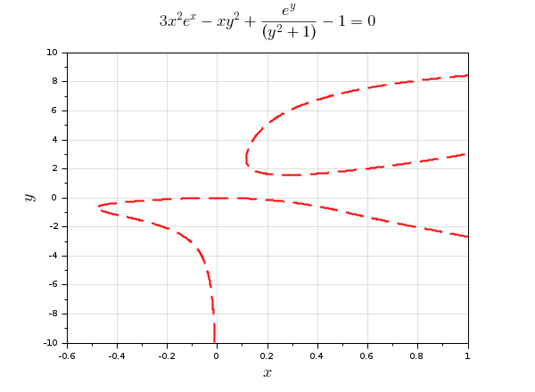
Using the default x_grid, a plotting option, and some post-processing:
equation = "3*x^2*exp(x) - x*y^2 +  exp(y)/(y^2 + 1) = 1"
plotimplicit(equation, , -10:0.1:10, "r--")

// Increase the contours thickness afterwards:
gce().children.thickness = 2;

// Setting titles and grids
title("$3x^2 e^x - x y^2 +  {{e^y}\over{(y^2 + 1)}} - 1 = 0$", "fontsize",4)
xgrid(color("grey"),1,7)
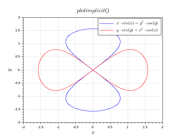
Overplotting:
clf
plotimplicit("x*sin(x) = y^2*cos(y)", [-2,2])

t1 = gca().title.text;
c1 = gce().children(1);
title("")

plotimplicit("y*sin(y) = x^2*cos(x)", [-2,2], ,"r")
t2 = gca().title.text;
c2 = gce().children(1);
title("$plotimplicit()$")

legend([c1 c2],[t1 t2]);
gce().font_size = 3;
xgrid(color("grey"),1,7)
See Also
- fsolve — résout un système d'équations non-linéaires
- contour2d — level curves on a 3D surface
- contour2di — calcule les courbes de niveau d'une surface
- contour2dm — compute level curves of a surface defined with a mesh
- LineSpec — to quickly customize the lines appearance in a plot
- GlobalProperty — customizes the objects appearance (curves, surfaces...) in a plot or surf command
- plot — 2D plot
History
| Version | Description |
| 6.1.0 | Function introduced. |
| Report an issue | ||
| << plot2d4 | 2d_plot | polarplot >> |