Scilab 6.1.0
Please note that the recommended version of Scilab is 2026.1.0. This page might be outdated.
See the recommended documentation of this function
hallchart
Draws a Hall chart
Syntax
sh = hallchart(modules)
sh = hallchart(modules, args)
sh = hallchart(modules, args, colors)
Arguments
- modules
- vector of real numbers: modules (in dB). Default values are computed according to the data bounds, whose default are [-4,3] for the Real axis and [-3 3] for the Imaginary one.
- args
- vector of real numbers: phases (in degree). Default values:
[-90 -60 -40 -30 -25 -20 -15 -12 12 15 20 25 30 40 60 90]° - colors
- vector of 1 or 2 components specifying the colors of the isogain and isophase
sets of curves. To choose the color for only one grid, set the other one to ""
or 0. If a single color is provided, it is used for both gains and phases.
colorsmay be specified either- by indices in the color map.
- named colors among the predefined ones.
- "#RRGGBB" hexadecimal case-insensitive strings starting with "#", like "#FA7B35".
- A 1x3 or 2x3 matrix of [r g b] intensities such that 0 <= r,g,b <= 1.
- sh
- Structure with 4 fields:
.phaseLines: vector of handles of isophase lines..phaseLines(i)is the line forargs(i)..phaseLabels: vector of handles of isophase labels..phaseLabels(i)is the label forargs(i)..gainLines: vector of handles of isogain lines..gainLines(i)is the line formodules(i)..gainLabels: vector of handles of isogain labels..gainLabels(i)is the label formodules(i).
Description
plots the Hall's chart: iso-module and iso-argument contours of
y/(1+y) in the real(y),
imag(y) plane
hallchart may be used in conjunction with
nyquist.
 | Datatips on isogain and isophase curves are customized. |
Examples
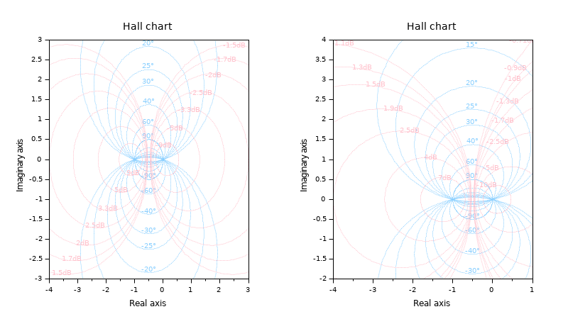
Charts in an empty default or empty preset axes: Note that default Hall chart titles are then set:
clf
// In a default axes
subplot(1,2,1)
hallchart();

// In a preset empty axes
subplot(1,2,2)
plotframe([-4 -2 1 4]) // xmin ymin ymax ymax
hallchart();
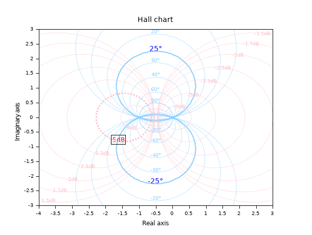
Customizing some elements of the grids and labels:
clf
h = hallchart();

// 5dB isogain
i = find(h.gainLabels.text=="5dB");
    // Customizing the label
set(h.gainLabels(i),"box","on","font_size",2,"font_foreground",color("red"));
    // Customizing the line
h.gainLines(i).thickness = 3;

// +/-25° isophases
i = grep(h.phaseLabels.text,"25°")
    // Customizing the labels
set(h.phaseLabels(i),"font_size",3,"font_foreground",color("blue"));
    // Customizing the lines
set(h.phaseLines(i), "thickness",2,"line_style",1);
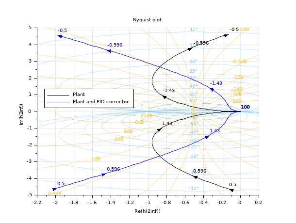
Background of a Nyquist diagram
Note that pre-existing titles are kept.s = %s; Plant = syslin('c', 16000/((s+1)*(s+10)*(s+100))); //two degree of freedom PID [tau, xsi] = (0.2, 1.2); PID = syslin('c',(1/(2*xsi*tau*s))*(1+2*xsi*tau*s+tau^2*s^2)); clf nyquist([Plant;Plant*PID], 0.5, 100, ["Plant";"Plant and PID corrector"]); mod = [12 6 3 2 1 0.5 0.2 0.1 -6 -3 -2 -1 -0.5 -0.2 -0.1]; hallchart(mod,, ["goldenrod1" ""]); // Move the caption to avoid hiding data Leg = gca().children(1); set(Leg,"legend_location","by_coordinates","position",[0.15 0.4]);
See also
- nicholschart — Nichols chart
- nyquist — nyquist plot
- black — Black-Nichols diagram of a linear dynamical system
- color_list — liste des noms de couleurs prédéfinies
History
| Version | Description |
| 6.1.0 |
|
| Report an issue | ||
| << gainplot | Domaine de fréquence | nicholschart >> |