Please note that the recommended version of Scilab is 2026.1.0. This page might be outdated.
See the recommended documentation of this function
histc
ヒストグラムを計算
呼び出し手順
h = histc(n, data)
h = histc(x, data)
h = histc(.., normalization)
引数
- n
正の整数 (クラスの数)
- x
クラスを定義する漸増ベクトル (
xには最低2つの要素があります)- data
ベクトル (解析対象のデータ)
- h
If
normalizationis %T: Probability densities on the bins defined bynorx, such that the bins areas are proportionnal to their populations.If
normalizationis %F: Numbers of elements in the bins.
- normalization
スカラー論理値 (デフォルト %T), setting the type of output (see
h).
説明
この関数は,クラスxによりdataベクトルの
ヒストグラムを計算します.
xではなくクラスの数 nが指定された場合,等間隔で
x(1) = min(data) < x(2) = x(1) + dx < ... < x(n+1) = max(data)
(ただし, dx = (x(n+1)-x(1))/n)となるクラスが選択されます.
クラスはC1 = [x(1), x(2)] および Ci = ( x(i), x(i+1)]
(i >= 2)で定義されます.
Nmaxはdataの総数 (Nmax = length(data)),
NiはCiに含まれるdata要素の数,
Ciにおけるxのヒストグラムの値は,
"normalized"が選択された場合は
Ni/(Nmax (x(i+1)-x(i))) となり,
そうでない場合は単にNiとなります.
正規化が行われた際,ヒストグラムは以下を確認します:

x(1)<=min(data) および max(data) <= x(n+1) の場合
例
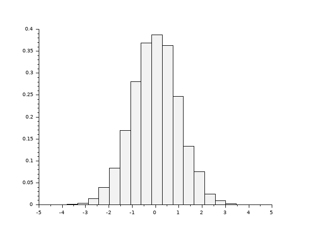
- 例 #1: ガウス乱数標本のヒストグラム周辺の変化
// ガウス乱数標本
d = rand(1, 10000, 'normal');
h = histc(20, d, normalization=%f);
sum(h)   // = 10000
// グラフィック表現を示すためにhistplotを使用
clf(); histplot(20, d, normalization=%f);

// Normalized histogram (probability density)
h = histc(20, d);
dx = (max(d)-min(d))/20;  sum(h)*dx   // = 1
clf(); histplot(20, d);
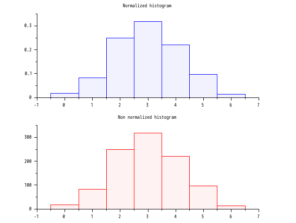
- 例 #2: 二項(B(6,0.5)) 乱数標本のヒストグラム
d = grand(1000,1,"bin", 6, 0.5);
c = linspace(-0.5,6.5,8);
clf()

subplot(2,1,1)
h = histc(c, d);
histplot(c, d, style=2);
xtitle(_("Normalized histogram"))

subplot(2,1,2)
h = histc(c, d, normalization=%f);
histplot(c, d, normalization=%f, style=5);
xtitle(_("Non normalized histogram"))
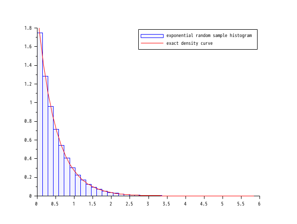
- 例 #3: 指数乱数標本のヒストグラム
lambda = 2;
X = grand(100000,1,"exp", 1/lambda);
Xmax = max(X);
h = histc(40, X);

clf()
histplot(40, X, style=2);
x = linspace(0, max(Xmax), 100)';
plot2d(x, lambda*exp(-lambda*x), strf="000", style=5)
legend([_("exponential random sample histogram") _("exact density curve")]);
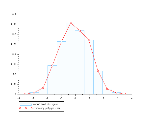
- 例 #4: ガウス乱数標本の周波数ポリゴンチャートとヒストグラム
n = 10;
data = rand(1, 1000, "normal");
h = histc(n, data);

clf(); histplot(n, data, style=12, polygon=%t);
legend([_("normalized histogram") _("frequency polygon chart")], "lower_caption");
参照
履歴
| バージョン | 記述 |
| 5.5.0 | Introduction |
| Report an issue | ||
| << covar | Descriptive Statistics | median >> |