Please note that the recommended version of Scilab is 2026.1.0. This page might be outdated.
See the recommended documentation of this function
leastsq
Solves non-linear least squares problems
Syntax
fopt=leastsq(fun, x0)
fopt=leastsq(fun, x0)
fopt=leastsq(fun, dfun, x0)
fopt=leastsq(fun, cstr, x0)
fopt=leastsq(fun, dfun, cstr, x0)
fopt=leastsq(fun, dfun, cstr, x0, algo)
fopt=leastsq([iprint], fun [,dfun] [,cstr],x0 [,algo],[df0,[mem]],[stop])
[fopt,xopt] = leastsq(...)
[fopt,xopt,gopt] =  = leastsq(...)
Arguments
- fopt
value of the function
f(x)=||fun(x)||^2atxopt- xopt
best value of
xfound to minimize||fun(x)||^2- gopt
gradient of
fatxopt- fun
a scilab function or a list defining a function from
R^ntoR^m(see more details in DESCRIPTION).- x0
real vector (initial guess of the variable to be minimized).
- dfun
a scilab function or a string defining the Jacobian matrix of
fun(see more details in DESCRIPTION).- cstr
bound constraints on
x. They must be introduced by the string keyword'b'followed by the lower boundbinfthen by the upper boundbsup(socstrappears as'b',binf,bsupin the syntax). Those bounds are real vectors with same dimension thanx0(-%inf and +%inf may be used for dimension which are unrestricted).- algo
a string with possible values:
'qn'or'gc'or'nd'. These strings stand for quasi-Newton (default), conjugate gradient or non-differentiable respectively. Note that'nd'does not accept bounds onx.- iprint
scalar argument used to set the trace mode.
iprint=0nothing (except errors) is reported,iprint=1initial and final reports,iprint=2adds a report per iteration,iprint>2add reports on linear search. Warning, most of these reports are written on the Scilab standard output.- df0
real scalar. Guessed decreasing of
||fun||^2at first iteration. (df0=1is the default value).- mem
integer, number of variables used to approximate the Hessian (second derivatives) of
fwhenalgo='qn'. Default value is 10.- stop
sequence of optional parameters controlling the convergence of the algorithm. They are introduced by the keyword
'ar', the sequence being of the form'ar',nap, [iter [,epsg [,epsf [,epsx]]]]- nap
maximum number of calls to
funallowed.- iter
maximum number of iterations allowed.
- epsg
threshold on gradient norm.
- epsf
threshold controlling decreasing of
f- epsx
threshold controlling variation of
x. This vector (possibly matrix) of same size asx0can be used to scalex.
Description
The leastsq function
solves the problem

where f is a function from
R^n to R^m.
Bound constraints cab be imposed on x.
How to provide fun and dfun
fun can be a scilab function (case
1) or a fortran or a C routine linked to scilab (case 2).
- case 1:
When
funis a Scilab function, its calling sequence must be:In the case where the cost function needs extra parameters, its header must be:y=fun(x)
In this case, we providey=f(x,a1,a2,...)
funas a list, which containslist(f,a1,a2,...).- case 2:
When
funis a Fortran or C routine, it must belist(fun_name,m[,a1,a2,...])in the syntax ofleastsq, wherefun_nameis a 1-by-1 matrix of strings, the name of the routine which must be linked to Scilab (see link). The header must be, in Fortran:and in C:subroutine fun(m, n, x, params, y) integer m,n double precision x(n), params(*), y(m)
wherevoid fun(int *m, int *n, double *x, double *params, double *y)
nis the dimension of vectorx,mthe dimension of vectory, withy=fun(x), andparamsis a vector which contains the optional parametersa1, a2, .... Each parameter may be a vector, for instance ifa1has 3 components, the description ofa2begin fromparams(4)(in fortran), and fromparams[3](in C). Note that even iffundoes not need supplementary parameters you must anyway write the fortran code with aparamsargument (which is then unused in the subroutine core).
By default, the algorithm uses a finite difference approximation
of the Jacobian matrix.
The Jacobian matrix can be provided by defining the function
dfun, where to the
optimizer it may be given as a usual scilab function or
as a fortran or a C routine linked to scilab.
- case 1:
when
dfunis a scilab function, its calling sequence must be:wherey=dfun(x)y(i,j)=dfi/dxj. If extra parameters are required byfun, i.e. if argumentsa1,a2,...are required, they are passed also todfun, which must have headerNote that, even ify=dfun(x,a1,a2,...)dfunneeds extra parameters, it must appear simply asdfunin the syntax ofleastsq.- case 2:
When
dfunis defined by a Fortran or C routine it must be a string, the name of the function linked to Scilab. The calling sequences must be, in Fortran:in C:subroutine dfun(m, n, x, params, y) integer m,n double precision x(n), params(*), y(m,n)
In the C casevoid fun(int *m, int *n, double *x, double *params, double *y)y(i,j)=dfi/dxjmust be stored iny[m*(j-1)+i-1].
Remarks
Like datafit,
leastsq is a front end onto the optim function. If you want to try the
Levenberg-Marquard method instead, use lsqrsolve.
A least squares problem may be solved directly with the optim function ; in this case the function NDcost may be useful to compute the derivatives (see the NDcost help page which provides a simple example for parameters identification of a differential equation).
Examples
We will show different calling possibilities of leastsq on one (trivial) example which is non linear but does not really need to be solved with leastsq (applying log linearizes the model and the problem may be solved with linear algebra). In this example we look for the 2 parameters x(1) and x(2) of a simple exponential decay model (x(1) being the unknown initial value and x(2) the decay constant):
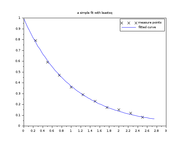
function y=yth(t, x)
   y  = x(1)*exp(-x(2)*t)
endfunction

// we have the m measures (ti, yi):
m = 10;
tm = [0.25, 0.5, 0.75, 1.0, 1.25, 1.5, 1.75, 2.0, 2.25, 2.5]';
ym = [0.79, 0.59, 0.47, 0.36, 0.29, 0.23, 0.17, 0.15, 0.12, 0.08]';
// measure weights (here all equal to 1...)
wm = ones(m,1);

// and we want to find the parameters x such that the model fits the given
// data in the least square sense:
//
//  minimize  f(x) = sum_i  wm(i)^2 ( yth(tm(i),x) - ym(i) )^2

// initial parameters guess
x0 = [1.5 ; 0.8];

// in the first examples, we define the function fun and dfun
// in scilab language
function e=myfun(x, tm, ym, wm)
   e = wm.*( yth(tm, x) - ym )
endfunction

function g=mydfun(x, tm, ym, wm)
   v = wm.*exp(-x(2)*tm)
   g = [v , -x(1)*tm.*v]
endfunction

// now we could call leastsq:

// 1- the simplest call
[f,xopt, gopt] = leastsq(list(myfun,tm,ym,wm),x0)

// 2- we provide the Jacobian
[f,xopt, gopt] = leastsq(list(myfun,tm,ym,wm),mydfun,x0)

// a small graphic (before showing other calling features)
tt = linspace(0,1.1*max(tm),100)';
yy = yth(tt, xopt);
scf();
plot(tm, ym, "kx")
plot(tt, yy, "b-")
legend(["measure points", "fitted curve"]);
xtitle("a simple fit with leastsq")

// 3- how to get some information (we use iprint=1)
[f,xopt, gopt] = leastsq(1,list(myfun,tm,ym,wm),mydfun,x0)

// 4- using the conjugate gradient (instead of quasi Newton)
[f,xopt, gopt] = leastsq(1,list(myfun,tm,ym,wm),mydfun,x0,"gc")

// 5- how to provide bound constraints (not useful here !)
xinf = [-%inf,-%inf];
xsup = [%inf, %inf];
// without Jacobian:
[f,xopt, gopt] = leastsq(list(myfun,tm,ym,wm),"b",xinf,xsup,x0)
// with Jacobian :
[f,xopt, gopt] = leastsq(list(myfun,tm,ym,wm),mydfun,"b",xinf,xsup,x0)

// 6- playing with some stopping parameters of the algorithm
//    (allows only 40 function calls, 8 iterations and set epsg=0.01, epsf=0.1)
[f,xopt, gopt] = leastsq(1,list(myfun,tm,ym,wm),mydfun,x0,"ar",40,8,0.01,0.1)
Examples with compiled functions
Now we want to define fun and dfun in Fortran, then in C. Note that the "compile and link to scilab" method used here is believed to be OS independent (but there are some requirements, in particular you need a C and a fortran compiler, and they must be compatible with the ones used to build your scilab binary).
Let us begin by an example with fun and dfun in fortran
// 7-1/ Let 's Scilab write the fortran code (in the TMPDIR directory):
f_code = ["      subroutine myfun(m,n,x,param,f)"
          "*     param(i) = tm(i), param(m+i) = ym(i), param(2m+i) = wm(i)"
          "      implicit none"
          "      integer n,m"
          "      double precision x(n), param(*), f(m)"
          "      integer i"
          "      do i = 1,m"
          "         f(i) = param(2*m+i)*( x(1)*exp(-x(2)*param(i)) - param(m+i) )"
          "      enddo"
          "      end ! subroutine fun"
          ""
          "      subroutine mydfun(m,n,x,param,df)"
          "*     param(i) = tm(i), param(m+i) = ym(i), param(2m+i) = wm(i)"
          "      implicit none"
          "      integer n,m"
          "      double precision x(n), param(*), df(m,n)"
          "      integer i"
          "      do i = 1,m"
          "         df(i,1) =  param(2*m+i)*exp(-x(2)*param(i))"
          "         df(i,2) = -x(1)*param(i)*df(i,1)"
          "      enddo"
          "      end ! subroutine dfun"];
cd TMPDIR;
mputl(f_code,TMPDIR+'/myfun.f')

// 7-2/ compiles it. You need a fortran compiler !
names = ["myfun" "mydfun"]
flibname = ilib_for_link(names,"myfun.f",[],"f");

// 7-3/ link it to scilab (see link help page)
link(flibname,names,"f")

// 7-4/ ready for the leastsq call: be carreful do not forget to
//      give the dimension m after the routine name !
[f,xopt, gopt] = leastsq(list("myfun",m,tm,ym,wm),x0)  // without Jacobian
[f,xopt, gopt] = leastsq(list("myfun",m,tm,ym,wm),"mydfun",x0) // with Jacobian
Last example: fun and dfun in C.
// 8-1/ Let 's Scilab write the C code (in the TMPDIR directory):
c_code = ["#include <math.h>"
          "void myfunc(int *m,int *n, double *x, double *param, double *f)"
          "{"
          "  /*  param[i] = tm[i], param[m+i] = ym[i], param[2m+i] = wm[i] */"
          "  int i;"
          "  for ( i = 0 ; i < *m ; i++ )"
          "    f[i] = param[2*(*m)+i]*( x[0]*exp(-x[1]*param[i]) - param[(*m)+i] );"
          "  return;"
          "}"
          ""
          "void mydfunc(int *m,int *n, double *x, double *param, double *df)"
          "{"
          "  /*  param[i] = tm[i], param[m+i] = ym[i], param[2m+i] = wm[i] */"
          "  int i;"
          "  for ( i = 0 ; i < *m ; i++ )"
          "    {"
          "      df[i] = param[2*(*m)+i]*exp(-x[1]*param[i]);"
          "      df[i+(*m)] = -x[0]*param[i]*df[i];"
          "    }"
          "  return;"
          "}"];

mputl(c_code,TMPDIR+'/myfunc.c')

// 8-2/ compiles it. You need a C compiler !
names = ["myfunc" "mydfunc"]
clibname = ilib_for_link(names,"myfunc.c",[],"c");

// 8-3/ link it to scilab (see link help page)
link(clibname,names,"c")

// 8-4/ ready for the leastsq call
[f,xopt, gopt] = leastsq(list("myfunc",m,tm,ym,wm),"mydfunc",x0)
See also
- lsqrsolve — minimize the sum of the squares of nonlinear functions, levenberg-marquardt algorithm
- optim — non-linear optimization routine
- NDcost — generic external for optim computing gradient using finite differences
- datafit — Parameter identification based on measured data
- external — objeto Scilab, função ou rotina externa
- qpsolve — linear quadratic programming solver
| Report an issue | ||
| << datafit | Nonlinear Least Squares | lsqrsolve >> |