dae

引数

initial

列ベクトル. x0または [x0;xdot0] とします. ただし, x0は 初期時刻t0における状態量の値, ydot0は状態量の微分の初期値 またはその推定値(下記参照)です.

t0

実数, 初期時刻.

t

実数のスカラーまたはベクトル. 解を計算する時刻を指定します. %DAEOPTIONS(2)=1 と設定することにより DAEの各ステップで解が得られることに注意してください.

atol

実数のスカラーまたはx0と同じ大きさの 列ベクトル. 解の絶対許容誤差. atolがベクトルの場合, 状態量の各要素毎に許容誤差が指定されます.

rtol

実数のスカラーまたはx0と同じ大きさの 列ベクトル. 解の相対許容誤差. rtolがベクトルの場合, 状態量の各要素毎に許容誤差が指定されます.

res

外部ルーチン. g(t,y,ydot)の値を計算します. 以下のようになります

Scilab関数

この場合, その呼出し手順を [r,ires]=res(t,x,xdot) とする 必要があり,res は 残差r=g(t,x,xdot) とエラーフラグ iresを返す必要があります. resがrの計算に 成功した場合にはires = 0, (t,x,xdot)のローカルな残差が定義されない 場合には =-1, パラメータが許容範囲外の場合は =-2 となります.

リスト

外部ルーチンのこの形式は 関数にパラメータを指定する際に使用されます. 以下のような形式とします:

list(res,p1,p2,...)

ただし,ここで関数resの呼び出し手順は以下のようになります

r=res(t,y,ydot,p1,p2,...)

この場合もres は (t,x,xdot,x1,x2,...)の関数として残差の値を返し, p1,p2,... は関数のパラメータです.

文字列

CまたはFortranルーチンの名前を指します. <r_name> が指定した名前であると仮定します.

• Fortranの呼出し手順は以下のようにします

  <r_name>(t,x,xdot,res,ires,rpar,ipar)

  double precision t,x(*),xdot(*),res(*),rpar(*)

  integer ires,ipar(*)

• Cの呼出し手順は以下のようにします

  C2F(<r_name>)(double *t, double *x, double *xdot, double *res, integer *ires, double *rpar, integer *ipar)

ただし,

• t はカレントの時刻

• xは状態量の配列

• xdot は状態量の微分の配列

• res は残差の配列

• iresは実行インジケータ

• rpar は浮動小数点数の パラメータ値の配列で, 必要ですが dae 関数により 設定できないもの

• ipar は整数の パラメータ値の配列で, 必要ですが dae 関数により 設定できないもの

jac

外部ルーチン. 指定したパラメータの値 cjを用いて dg/dx+cj*dg/dxdotの値を計算します. 以下のようになります

Scilab関数

呼出し手順を r=jac(t,x,xdot,cj) とする 必要があり, jac関数は r=dg(t,x,xdot)/dy+cj*dg(t,x,xdot)/dxdot を返す必要があります. ただし,cjは実数スカラーです.

リスト

外部ルーチンのこの形式は 関数にパラメータを指定する際に使用されます. 以下のような形式とします:

list(jac,p1,p2,...)

ただしこの場合の関数jacの呼び出し手順は 以下となります

r=jac(t,x,xdot,p1,p2,...)

この場合でもjac は, (t,x,xdot,cj,p1,p2,...)の関数として dg/dx+cj*dg/dxdotを返します.

文字列

CまたはFortranルーチンの名前を指します. <j_name> が指定した名前であると仮定します.

• Fortranの呼出し手順は以下のようにします

  <j_name>(t, x, xdot, r, cj, ires, rpar, ipar)

  double precision t, x(*), xdot(*), r(*), ci, rpar(*)

  integer ires, ipar(*)

• Cの呼出し手順は以下のようにします

  C2F(<j_name>)(double *t, double *x, double *xdot, double *r, double *cj,

  integer *ires, double *rpar, integer *ipar)

ただし t, x, xdot, ires, rpar, ipar は上記と似た定義を有し, r は配列の結果です.

surface

外部ルーチン. ng個の要素を有する列ベクトル surface(t,x)の値を計算します. 各要素は面(surface)を定義します.

Scilab関数

その呼び出し手順はr=surface(t,x)とする 必要があり,この関数は ng個の要素を有する ベクトルを返す必要があります.

リスト

外部ルーチンのこの形式は 関数にパラメータを指定する際に使用されます. 以下のような形式とします:

list(surface,p1,p2,...)

ただしこの場合の関数surfaceの呼び出し手順は 以下となります

r=surface(t,x,p1,p2,...)

文字列

CまたはFortranルーチンの名前を指します. <s_name> が指定した名前であると仮定します,

• Fortranの呼出し手順は以下のようにします

  <r_name>(nx, t, x, ng, r, rpar, ipar)

  double precision t, x(*), r(*), rpar(*)

  integer nx, ng,ipar(*)

• Cの呼出し手順は以下のようにします

  C2F(<r_name>)(double *t, double *x, double *xdot, double *r, double *cj,

  integer *ires, double *rpar, integer *ipar)

ただし,t, x, rpar, ipar は 上記と同じ定義を有し,ng は surfacesの数, nx は状態量の次元, r は結果の配列です.

rd

2個のエントリ [times num]を有するベクトル. times は面が交差した時刻の値, num は交差した面の数です

pjac

外部 (関数, リストまたは文字列). daskr参照.

psol

外部 (関数, リストまたは文字列). daskr参照.

hd

実数のベクトル, dae コンテキストを保持する出力. (ホットスタートで)積分を再開するための入力引数として使用可能です.

y

実数の行列. %DAEOPTIONS(2)=1 の場合, 各列 はベクトル [t;x(t);xdot(t)] です. ただし, t は解が計算された時刻です. それ以外の場合, y はベクトル [x(t);xdot(t)]です.

説明

dae 関数は, 陰的な微分方程式積分用に設計された dassl および dasrt 関数の上位に構築されたゲートウエイです.

オプション "root" は dasrt ルーチンをコールし, "root2" は daskrをコールします.

g(t,x,xdot)=0
x(t0)=x0  および   xdot(t0)=xdot0

initial引数にxdot0 が指定されない場合, dae関数は g(t,x0,xdot0)=0 を解くことによりこれを計算しようとします.

xdot0 が initial引数で指定された場合, g(t,x0,xdot0)=0を満たす互換性がある微係数または近似値の どちらかとなります. 後者の場合, %DAEOPTIONS(7) を 1 に設定する必要があります.

Scilab および C でコーディングされた外部ルーチンを使用する詳細な例については, modules/differential_equations/tests/unit_tests/dassldasrt.tst および modules/differential_equations/tests/unit_tests/daskr.tst で提供されています.

例

例 #1: dassl (求解なし)

// Scilabコードを使用する例
function [r, ires]=chemres(t, y, yd)
    r(1) = -0.04*y(1) + 1d4*y(2)*y(3) - yd(1);
    r(2) =  0.04*y(1) - 1d4*y(2)*y(3) - 3d7*y(2)*y(2) - yd(2);
    r(3) =       y(1) +     y(2)      + y(3)-1;
    ires =  0;
endfunction
function pd=chemjac(x, y, yd, cj)
    pd=[-0.04-cj , 1d4*y(3)               , 1d4*y(2);
         0.04    ,-1d4*y(3)-2*3d7*y(2)-cj ,-1d4*y(2);
         1       , 1                      , 1       ]
endfunction

x0=[1; 0; 0];
xd0=[-0.04; 0.04; 0];
t=[1.d-5:0.02:.4, 0.41:.1:4, 40, 400, 4000, 40000, 4d5, 4d6, 4d7, 4d8, 4d9, 4d10];

y=dae([x0,xd0],0,t,chemres);// 指定した観測時刻での点を返す

%DAEOPTIONS=list([],1,[],[],[],0,0); // dae メッシュ点を返すかどうかを確認
y=dae([x0,xd0],0,4d10,chemres); // ヤコビアン指定なし
y=dae([x0,xd0],0,4d10,chemres,chemjac); // ヤコビアン指定あり

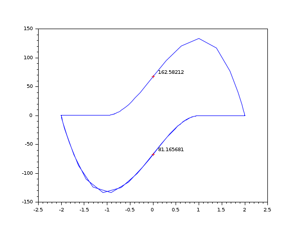
例 #2: dasrt ("root")

// C コードの例 (Cコンパイラが必要) --------------------------------------------------
bOK = haveacompiler();
if bOK <> %t
    [btn] = messagebox(["You need a C compiler for this example."; "Execution of this example is canceled."], "Software problem", 'info');
    return
end

//-1- Cコードを TMPDIR に作成 - Vanderpol 方程式, 陰形式
code=['#include <math.h>'
      'void res22(double *t,double *y,double *yd,double *res,int *ires,double *rpar,int *ipar)'
      '{res[0] = yd[0] - y[1];'
      ' res[1] = yd[1] - (100.0*(1.0 - y[0]*y[0])*y[1] - y[0]);}'
      ' '
      'void jac22(double *t,double *y,double *yd,double *pd,double *cj,double *rpar,int *ipar)'
      '{pd[0]=*cj - 0.0;'
      ' pd[1]=    - (-200.0*y[0]*y[1] - 1.0);'
      ' pd[2]=    - 1.0;'
      ' pd[3]=*cj - (100.0*(1.0 - y[0]*y[0]));}'
      ' '
      'void gr22(int *neq, double *t, double *y, int *ng, double *groot, double *rpar, int *ipar)'
      '{ groot[0] = y[0];}']
mputl(code,TMPDIR+'/t22.c')
//-2- コンパイルの後,ロード
ilib_for_link(['res22' 'jac22' 'gr22'],'t22.c',[],'c',[],TMPDIR+'/t22loader.sce');
exec(TMPDIR+'/t22loader.sce')
//-3- 実行
rtol=[1.d-6;1.d-6];atol=[1.d-6;1.d-4];
t0=0;y0=[2;0];y0d=[0;-2];t=[20:20:200];ng=1;
//簡単なシミュレーション
t=0:0.003:300;
yy=dae([y0,y0d],t0,t,atol,rtol,'res22','jac22');
clf();plot(yy(1,:),yy(2,:))
//find first point where yy(1)=0
[yy,nn,hotd]=dae("root",[y0,y0d],t0,300,atol,rtol,'res22','jac22',ng,'gr22');
plot(yy(1,1),yy(2,1),'r+')
xstring(yy(1,1)+0.1,yy(2,1),string(nn(1)))

//次の点までホットリスタート
t01=nn(1);
[pp,qq]=size(yy);
y01=yy(2:3,qq);y0d1=yy(3:4,qq);
[yy,nn,hotd]=dae("root",[y01,y0d1],t01,300,atol,rtol,'res22','jac22',ng,'gr22',hotd);
plot(yy(1,1),yy(2,1),'r+')
xstring(yy(1,1)+0.1,yy(2,1),string(nn(1)));
cd(previous_dir);

例 #3: daskr ("root2"), デフォルトの 'psol' および 'pjac' ルーチンを使用

// Example with C code (C compiler needed)
//--------------------------------------------------
bOK = haveacompiler();
if bOK <> %t
    [btn] = messagebox(["You need a C compiler for this example."; "Execution of this example is canceled."], "Software problem", 'info');
    return
end

//-1- Create the C codes in TMPDIR - Vanderpol equation, implicit form
code = ['#include <math.h>'
      'void res22(double *t, double *y, double *yd, double *res, int *ires, double *rpar, int *ipar)'
      '{res[0] = yd[0] - y[1];'
      ' res[1] = yd[1] - (100.0*(1.0 - y[0]*y[0])*y[1] - y[0]);}'
      ' '
      'void jac22(double *t, double *y, double *yd, double *pd, double *cj, double *rpar, int *ipar)'
      '{pd[0] = *cj - 0.0;'
      ' pd[1] =     - (-200.0*y[0]*y[1] - 1.0);'
      ' pd[2] =     - 1.0;'
      ' pd[3] = *cj - (100.0*(1.0 - y[0]*y[0]));}'
      ' '
      'void gr22(int *neq, double *t, double *y, int *ng, double *groot, double *rpar, int *ipar)'
      '{ groot[0] = y[0];}']
previous_dir = pwd();
cd TMPDIR;
mputl(code, 't22.c')

//-2- Compile and load them
ilib_for_link(['res22' 'jac22' 'gr22'], 't22.c', [], 'c', [], 't22loader.sce');
exec('t22loader.sce')

//-3- Run
rtol = [1.d-6; 1.d-6];
atol = [1.d-6; 1.d-4];
t0 = 0; t = [20:20:200];
y0 = [2; 0]; y0d = [0; -2];
ng = 1;

// Simple simulation
t = 0:0.003:300;
yy = dae([y0, y0d], t0, t, atol, rtol, 'res22', 'jac22');
clf(); plot(yy(1, :), yy(2, :))
// Find first point where yy(1) = 0
%DAEOPTIONS = list([] , 0, [], [], [], 0, [], 1, [], 0, 1, [], [], 1);
[yy, nn, hotd] = dae("root2", [y0, y0d], t0, 300, atol, rtol, 'res22', 'jac22', ng, 'gr22', 'psol1', 'pjac1');
plot(yy(1, 1), yy(2, 1), 'r+')
xstring(yy(1, 1)+0.1, yy(2, 1), string(nn(1)));

// Hot restart for next point
t01 = nn(1);
[pp, qq] = size(yy);
y01 = yy(2:3, qq); y0d1 = yy(3:4, qq);
[yy, nn, hotd] = dae("root2", [y01, y0d1], t01, 300, atol, rtol, 'res22', 'jac22', ng, 'gr22', 'psol1', 'pjac1', hotd);
plot(yy(1, 1), yy(2, 1), 'r+')
xstring(yy(1, 1)+0.1, yy(2, 1), string(nn(1)));
cd(previous_dir);

参照

• ode — 常微分方程式ソルバ
• daeoptions — daeソルバのオプションを設定
• dassl — 微分代数方程式
• dasrt — ゼロ交差するDAE
• daskr — ゼロ交差を有するDAEソルバー
• impl — 微分代数方程式
• fort — Fortran or C user routines call
• link — dynamic linker
• external — Scilabオブジェクト, 外部関数またはルーチン