Scilab 5.5.2
- Scilabヘルプ
- Graphics
- 2d_plot
- LineSpec
- Matplot
- Matplot1
- Matplot_properties
- Sfgrayplot
- Sgrayplot
- champ
- champ1
- champ_properties
- comet
- contour2d
- contour2di
- contourf
- errbar
- fchamp
- fcontour2d
- fec
- fec_properties
- fgrayplot
- fplot2d
- grayplot
- grayplot_properties
- graypolarplot
- histplot
- paramfplot2d
- plot
- plot2d
- plot2d1
- plot2d2
- plot2d3
- plot2d4
- polarplot
- contour2dm
Please note that the recommended version of Scilab is 2026.1.0. This page might be outdated.
See the recommended documentation of this function
Sfgrayplot
関数により定義された曲面の平滑化2次元カラープロット
呼び出し手順
Sfgrayplot(x, y, f, <opt_args>)

Sfgrayplot(x, y, f [,strf, rect, nax, zminmax, colminmax, mesh, colout])
引数
説明
Sfgrayplot は
fgrayplot と同じですが,プロットが平滑化されるところが
異なります. 平滑化には関数 fec が使用されます.
面の描画の際には,以下のグリッド (ここでは n1=5,
n2=3)から構築された
一連の三角形上では線形であると仮定されます:
_____________

| /| /| /| /|

|/_|/_|/_|/_|

| /| /| /| /|

|/_|/_|/_|/_|
関数 colorbar は色スケールを参照する 際にも使用できます (しかし,最小値と最大値が既知(または計算する)必要があります).
Sfgrayplotの代わりに, Sgrayplot を 使用することができ,若干高速化される可能性があります.
デモを参照するにはコマンド Sfgrayplot() を入力してください.
例
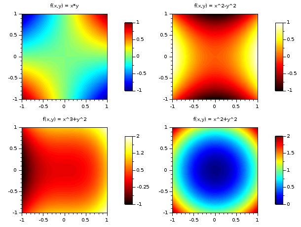
// 例 #1: 4 個の面をプロット

function z=surf1(x, y), z=x*y, endfunction

function z=surf2(x, y), z=x^2-y^2, endfunction

function z=surf3(x, y), z=x^3+y^2, endfunction

function z=surf4(x, y), z=x^2+y^2, endfunction

clf()

set(gcf(),"color_map",[jetcolormap(64);hotcolormap(64)])

x = linspace(-1,1,60);

y = linspace(-1,1,60);

drawlater() ;

subplot(2,2,1)

  colorbar(-1,1,[1,64])

  Sfgrayplot(x,y,surf1,strf="041",colminmax=[1,64])

  xtitle("f(x,y) = x*y")

subplot(2,2,2)

  colorbar(-1,1,[65,128])

  Sfgrayplot(x,y,surf2,strf="041",colminmax=[65,128])

  xtitle("f(x,y) = x^2-y^2")

subplot(2,2,3)

  colorbar(-1,2,[65,128])

  Sfgrayplot(x,y,surf3,strf="041",colminmax=[65,128])

  xtitle("f(x,y) = x^3+y^2")

subplot(2,2,4)

  colorbar(0,2,[1,64])

  Sfgrayplot(x,y,surf4,strf="041",colminmax=[1,64])

  xtitle("f(x,y) = x^2+y^2")

drawnow() ;

show_window()
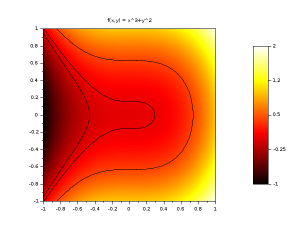
// 例 #2: surf3 をプロットしいくつかの等高線を追加

function z=surf3(x, y), z=x^3+y^2, endfunction

clf()

x = linspace(-1,1,60);

y = linspace(-1,1,60);

set(gcf(),"color_map",hotcolormap(128))

drawlater() ;

colorbar(-1,2)

Sfgrayplot(x,y,surf3,strf="041")

fcontour2d(x,y,surf3,[-0.1, 0.025, 0.4],style=[1 1 1],strf="000")

xtitle("f(x,y) = x^3+y^2")

drawnow() ;

show_window()
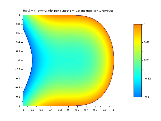
// 例 #3: surf3 をプロットし,プロットを -0.5<= z <= 1に制限するために

// オプションの引数 zminmax および colout を使用

function z=surf3(x, y), z=x^3+y^2, endfunction

clf()

x = linspace(-1,1,60);

y = linspace(-1,1,60);

set(gcf(),"color_map",jetcolormap(128))

drawlater() ;

zminmax = [-0.5 1]; colors=[32 96];

colorbar(zminmax(1),zminmax(2),colors)

Sfgrayplot(x, y, surf3, strf="041", zminmax=zminmax, colout=[0 0], colminmax=colors)

fcontour2d(x,y,surf3,[-0.5, 1],style=[1 1 1],strf="000")

xtitle("f(x,y) = x^3+y^2, with parts under z = -0.5 and upper z = 1 removed")

drawnow() ;

show_window()
参照
| Report an issue | ||
| << Matplot_properties | 2d_plot | Sgrayplot >> |