Please note that the recommended version of Scilab is 2026.1.0. This page might be outdated.
See the recommended documentation of this function
histc
calcule un histogramme
Séquence d'appel
[cf, ind] = histc(n, data [,normalization])
[cf, ind] = histc(x, data [,normalization])
Paramètres
- n
entier positif (nombre de classes)
- x
vecteur croissant définissant les classes (
xdoit avoir au moins 2 éléments)- data
vecteur (données à analyser)
- cf
vecteur représentant le nombre de valeurs de
datatombant dans les classes définies parnoux- ind
vecteur ou matrice de même taille que
data, représentant l'appartenance respective de chaque élément dedataaux classes définies parnoux- normalization
scalaire booléen.
normalization=%f (par défaut):cfreprésente le nombre total de points dans chaque classe,normalization=%t:cfreprésente le nombre de points dans chaque classe, relativement au nombre total de points
Description
Cette fonction calcule un histogramme du vecteur data d'après les classes
x. Quand le nombre de classes n est fourni
au lieu de x, les classes sont choisies également espacées et
x(1) = min(data) < x(2) = x(1) + dx < ... < x(n+1) = max(data)
avec dx = (x(n+1)-x(1))/n.
Les classes sont définies par C1 = [x(1), x(2)] et Ci = ( x(i), x(i+1)] pour i >= 2.
Si l'on note Nmax le nombre total de data (Nmax = length(data))
et Ni le nombre d'éléments de data tombant dans
Ci, la valeur de l'histogramme pour x dans
Ci est égal à Ni/(Nmax (x(i+1)-x(i))) quand
"normalized" est séléctionné et sinon, simplement égal à Ni.
Quand la normalisation a lieu, l'histogramme vérifie:

quand x(1)<=min(data) et max(data) <= x(n+1)
Exemples
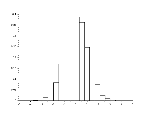
- Exemple #1: variations sur l'histogramme d'un échantillon gaussien N(0,1)
// L'échantillon aléatoire gaussien
d = rand(1, 10000, 'normal');

[cf, ind] = histc(20, d, normalization=%f)
// On utilise histplot pour avoir une représentation graphique
clf(); histplot(20, d, normalization=%f);

[cf, ind] = histc(20, d)
clf(); histplot(20, d);
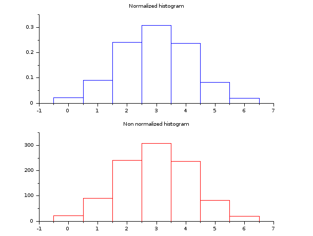
- Exemple #2: histogramme d'un échantillon de loi binomiale B(6,0.5)
d = grand(1000,1,"bin", 6, 0.5);
c = linspace(-0.5,6.5,8);
clf()
subplot(2,1,1)
[cf, ind] = histc(c, d)
histplot(c, d, style=2);
xtitle("Normalized histogram")
subplot(2,1,2)
[cf, ind] = histc(c, d, normalization=%f)
histplot(c, d, normalization=%f, style=5);
xtitle("Non normalized histogram")
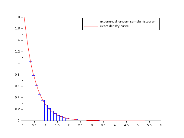
- Exemple #3: histogramme d'un échantillon de loi exponentielle E(lambda)
lambda = 2;
X = grand(100000,1,"exp", 1/lambda);
Xmax = max(X);
[cf, ind] = histc(40, X)
clf()
histplot(40, X, style=2);
x = linspace(0, max(Xmax), 100)';
plot2d(x, lambda*exp(-lambda*x), strf="000", style=5)
legend(["exponential random sample histogram" "exact density curve"]);
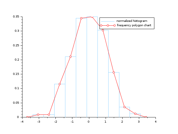
- Exemple #4: la fréquence polygonale et l'histogramme d'un échantillon gaussien
n = 10;
data = rand(1, 1000, "normal");
[cf, ind] = histc(n, data)
clf(); histplot(n, data, style=12, polygon=%t);
legend(["normalized histogram" "frequency polygon chart"]);
Voir aussi
History
| Version | Description |
| 5.5.0 | Introduction |
| Report an issue | ||
| << Descriptive Statistics | Descriptive Statistics | median >> |