Please note that the recommended version of Scilab is 2026.1.0. This page might be outdated.
See the recommended documentation of this function
karmarkar
Solves a linear optimization problem.
Calling Sequence
xopt=karmarkar(Aeq,beq,c)
xopt=karmarkar(Aeq,beq,c,x0)
xopt=karmarkar(Aeq,beq,c,x0,rtolf)
xopt=karmarkar(Aeq,beq,c,x0,rtolf,gam)
xopt=karmarkar(Aeq,beq,c,x0,rtolf,gam,maxiter)
xopt=karmarkar(Aeq,beq,c,x0,rtolf,gam,maxiter,outfun)
xopt=karmarkar(Aeq,beq,c,x0,rtolf,gam,maxiter,outfun,A,b)
xopt=karmarkar(Aeq,beq,c,x0,rtolf,gam,maxiter,outfun,A,b,lb)
xopt=karmarkar(Aeq,beq,c,x0,rtolf,gam,maxiter,outfun,A,b,lb,ub)
[xopt,fopt] = karmarkar(...)
[xopt,fopt,exitflag] = karmarkar(...)
[xopt,fopt,exitflag,iter] = karmarkar(...)
[xopt,fopt,exitflag,iter,yopt] = karmarkar(...)
Arguments
- Aeq
a n-by-p matrix of doubles, where
nis the number of linear equality constraints andpis the number of unknowns, the matrix in the linear equality constraints.- beq
a n-by-1 matrix of doubles, the right hand side of the linear equality constraint.
- c
a p-by-1 matrix of doubles, the linear part of the objective function.
- x0
a p-by-1 matrix of doubles, the initial guess (default
x0=[]). Ifx0==[], the karmarkar function automatically computes a feasible initial guess.- rtolf
a 1-by-1 matrix of doubles, a relative tolerance on
f(x)=c'*x(defaultrtolf=1.d-5).- gam
a 1-by-1 matrix of doubles, the scaling factor (default
gam=0.5). The scaling factor must satisfy0<gam<1.- maxiter
a 1-by-1 matrix of floating point integers, the maximum number of iterations (default
maxiter=200). The maximum number of iterations must be greater than 1.- outfun
a function or a list, the output function. See below for details.
- A
a ni-by-p matrix of doubles, the matrix of linear inequality constraints.
- b
a ni-by-1 matrix of doubles, the right-hand side of linear inequality constraints.
- lb
a p-by-1 matrix of doubles, the lower bounds.
- ub
a p-by-1 matrix of doubles, the upper bounds.
- xopt
a p-by-1 matrix of doubles, the solution.
- fopt
a 1-by-1 matrix of doubles, the objective function value at optimum, i.e.
fopt=c'*xopt.- exitflag
a 1-by-1 matrix of floating point integers, the status of execution. See below for details.
- iter
a 1-by-1 matrix of floating point integers, the number of iterations.
- yopt
a
structcontaining the dual solution. The structure yopt has four fields : ineqlin, eqlin, upper, lower. The fieldyopt.ineqlinis the Lagrange multiplier for the inequality constraints. The fieldyopt.eqlinis the Lagrange multiplier for the equality constraints. The fieldyopt.upperis the Lagrange multiplier for the upper bounds. The fieldyopt.loweris the Lagrange multiplier for the lower bounds.
Description
Computes the solution of linear programming problems.
This function has the two following modes.
If no inequality constraints and no bound is given (i.e. if
(A==[] & lb==[] & ub==[])), the function ensures that the variable is nonnegative.If any inequality constraints or any bound is given (i.e. if
(A<>[] or lb<>[] or ub<>[])), the function takes into account for this inequality or bound (and does not ensure that the variable is nonnegative).
If no inequality constraints and no bound is given
(i.e. if (A==[] & lb==[] & ub==[])),
solves the linear optimization problem:

If any inequality constraints or any bound is given
(i.e. if (A<>[] | lb<>[] | ub<>[])),
solves the linear optimization problem:

Any optional parameter equal to the empty matrix [] is replaced by
its default value.
The exitflag parameter allows to know why the algorithm
terminated.
exitflag = 1if algorithm converged.exitflag = 0if maximum number of iterations was reached.exitflag = -1if no feasible point was foundexitflag = -2if problem is unbounded.exitflag = -3if search direction became zero.exitflag = -4if algorithm stopped on user's request.
The output function outfun must have header
stop = outfun ( xopt , optimValues , state )
where
xopt is a p-by-1 matrix of double representing
the current point,
optimValues is a struct,
state is a 1-by-1 matrix of strings.
Here, stop is a 1-by-1 matrix of booleans,
which is %t if the algorithm must stop.
optimValues has the following fields:
optimValues.funccount: a 1-by-1 matrix of floating point integers, the number of function evaluationsoptimValues.fval: a 1-by-1 matrix of doubles, the best function valueoptimValues.iteration: a 1-by-1 matrix of floating point integers, the current iteration numberoptimValues.procedure: a 1-by-1 matrix of strings, the type of step performed.optimValues.dualgap: a 1-by-1 matrix of doubles, the duality gap, i.e.abs(yopt'*beq - fopt). At optimum, the duality gap is zero.
The optimValues.procedure field can have the following values.
If
optimValues.procedure="x0", then the algorithm is computing the initial feasible guessx0(phase 1).If
optimValues.procedure="x*", then the algorithm is computing the solution of the linear program (phase 2).
It might happen that the output function requires additionnal arguments to be evaluated.
In this case, we can use the following feature.
The function outfun can also be the list (outf,a1,a2,...).
In this case outf, the first element in the list, must have the header:
stop = outf ( xopt , optimValues , state , a1 , a2 , ... )
where the input arguments a1, a2, ...
will be automatically be appended at the end of the calling sequence.
Stopping rule
The stopping rule is based on the number of iterations, the relative tolerance on the function value, the duality gap and the user's output function.
In both the phase 1 and phase 2 of the algorithm, we check the duality gap and the boolean:
dualgap > 1.e5 * dualgapmin
where dualgap is the absolute value of the duality gap, and
dualgapmin is the minimum absolute duality gap measured during
this step of the algorithm.
The duality gap is computed from
dualgap = abs(yopt'*beq - fopt)
where yopt is the Lagrange multiplier, beq
is the right hand side of the inequality constraints and fopt
is the minimum function value attained in the current phase.
During the second phase of the algorithm (i.e. once x0 is
determined), the termination condition for the function value is based on the boolean:
where fprev is the previous function value,
fopt is the current function value and
rtolf is the relative tolerance on the function value.
Implementation notes
The implementation is based on the primal affine scaling algorithm, as discovered by Dikin in 1967, and then re-discovered by Barnes and Vanderbei et al in 1986.
If the scaling factor gam is closer to 1 (say gam=0.99,
for example), then the number of iterations may be lower.
Tsuchiya and Muramatsu proved that if an optimal solution exists, then, for any
gam lower than 2/3, the sequence converges to a point in the interior point of the optimal face.
Dikin proved convergence with gam=1/2.
Mascarenhas found two examples where the parameter gam=0.999 lets the
algorithm converge to a vertex which is not optimal, if the initial guess is chosen
appropriately.
Example #1
In the following example, we solve a linear optimization problem with 2 linear equality constraints and 3 unknowns. The linear optimization problem is

The following script solves the problem.
Aeq = [
1 -1 0
1  1 1
];
beq = [0;2];
c = [-1;-1;0];
x0 = [0.1;0.1;1.8];
[xopt,fopt,exitflag,iter,yopt]=karmarkar(Aeq,beq,c)
xstar=[1 1 0]'
The previous script produces the following output.
-->[xopt,fopt,exitflag,iter,yopt]=karmarkar(Aeq,beq,c)
 yopt  =
   ineqlin: [0x0 constant]
   eqlin: [2x1 constant]
   lower: [3x1 constant]
   upper: [3x1 constant]
 iter  =
    68.
 exitflag  =
    1.
 fopt  =
  - 1.9999898
 xopt  =
    0.9999949
    0.9999949
    0.0000102
We can explore the Lagrange multipliers by detailing each field of the yopt structure.
-->yopt.ineqlin
 ans  =
     []
-->yopt.eqlin
 ans  =
  - 6.483D-17
    1.
-->yopt.lower
 ans  =
  - 2.070D-10
  - 2.070D-10
    1.
-->yopt.upper
 ans  =
    0.
    0.
    0.
We can as well give the initial guess x0, as in the following script.
Aeq = [
1 -1 0
1  1 1
];
beq = [0;2];
c = [-1;-1;0];
x0 = [0.1;0.1;1.8];
[xopt,fopt,exitflag,iter,yopt]=karmarkar(Aeq,beq,c,x0)
In the case where we need more precision, we can reduce the relative tolerance on the function value. In general, reducing the tolerance increases the number of iterations.
-->[xopt,fopt,exitflag,iter]=karmarkar(Aeq,beq,c,[],1.e-5);
-->disp([fopt iter])
  - 1.9999898    68.
-->[xopt,fopt,exitflag,iter]=karmarkar(Aeq,beq,c,[],1.e-7);
-->disp([fopt iter])
  - 1.9999998    74.
-->[xopt,fopt,exitflag,iter]=karmarkar(Aeq,beq,c,[],1.e-9);
-->disp([fopt iter])
  - 2.    78.
Example #2
In the following example, we solve a linear optimization problem with 10 random linear equality constraints and 20 unknowns. The initial guess is chosen at random in the [0,1]^p range.
Inequality constraints
Consider the following linear program with inequality constraints.

c = [-20 -24]';
A = [
3 6
4 2
];
b = [60 32]';
xopt=karmarkar([],[],c,[],[],[],[],[],A,b)
The previous script produces the following output.
-->xopt=karmarkar([],[],c,[],[],[],[],[],A,b)
 xopt  =
    3.9999125
    7.9999912
With bounds
Consider the following linear optimization problem. The problem is used in the Scilab port of the Lipsol toolbox by Rubio Scola (example0.sce). The original Lipsol toolbox was created by Yin Zhang.

where S4 = sin(pi/4)/4 and E2 = exp(2).
c = [ 2; 5; -2.5];
S4 = sin(%pi/4)/4;
E2 = exp(2);
A = [
1  0 S4
E2 -1 -1
];
b = [ 5; 0];
lb = [ -2; 1   ; 0 ];
ub = [  2; %inf; 3 ];
xstar = [-2;1;3];
[xopt,fopt,exitflag,iter,yopt]=karmarkar([],[],c,[],[],[],[],[],A,b,lb,ub)
The previous script produces the following output.
-->[xopt,fopt,exitflag,iter,yopt]=karmarkar([],[],c,[],[],[],[],[],A,b,lb,ub)
    yopt  =
    ineqlin: [2x1 constant]
    eqlin: [0x0 constant]
    lower: [3x1 constant]
    upper: [3x1 constant]
    iter  =
    76.
    exitflag  =
    1.
    fopt  =
    - 6.4999482
    xopt  =
    - 1.9999914
    1.0000035
    2.9999931
Configuring an output function
It may be useful to configure a callback, so that we can customize the printed messages or create a plot. Consider the following linear optimization problem, which is presented on Wikipedia in Karmarkar's algorithm.

The following output function plots the current point and prints the iteration number, the value of the objective function.
function stop=myoutputfunction(xopt, optimValues, state)
    localmsg = gettext("Iter#%3.0f: %s (%s), "+..
        "f=%10.3e, x=[%s], gap=%10.3e\n")
    xstr = strcat(msprintf("%10.3e\n",xopt)'," ")
    mprintf(localmsg,optimValues.iteration,state,optimValues.procedure,..
        optimValues.fval,xstr,optimValues.dualgap)
    plot(xopt(1),xopt(2),"bo")
    stop = %f
endfunction
The following script defines the optimization problem and runs the optimization.
n=11;
A = [2*linspace(0,1,n)',ones(n,1)];
b = 1 + linspace(0,1,n)'.^2;
c=[-1;-1];
// Plot the constraints
scf();
for i = 1 : n
  plot(linspace(0,1,100),b(i)-A(i,1)*linspace(0,1,100),"b-")
end
// Run the optimization
xopt=karmarkar([],[],c,[],[],[],[],myoutputfunction,A,b);
// Plot the starting and ending points
plot(xopt(1),xopt(2),"k*")
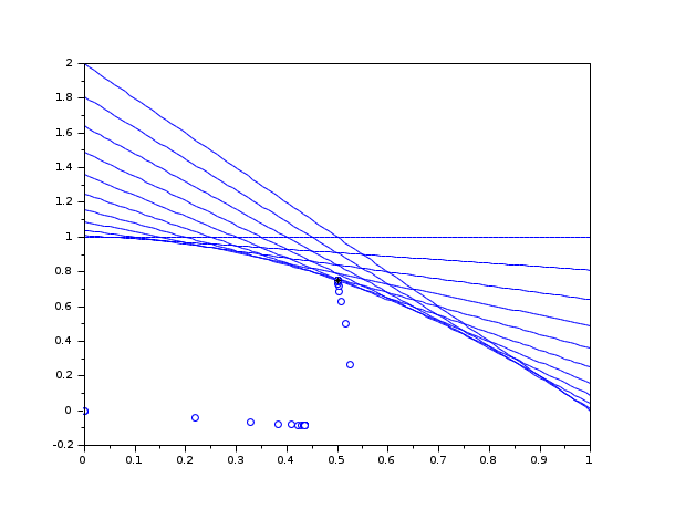
The previous script produces the following output and creates a graphics.
-->xopt=karmarkar([],[],c,[],[],[],[],myoutputfunction,A,b);
Iter#  0: init (x0), f=1.000e+000, x=[0.000e+000 0.000e+000], gap=Inf
Iter#  0: init (x0), f=1.000e+000, x=[0.000e+000 0.000e+000], gap=Inf
Iter#  1: init (x0), f=5.000e-001, x=[2.201e-001 -4.313e-002], gap=3.676e-001
Iter#  2: init (x0), f=2.500e-001, x=[3.283e-001 -6.512e-002], gap=2.140e-001
Iter#  3: init (x0), f=1.250e-001, x=[3.822e-001 -7.634e-002], gap=1.161e-001
Iter#  4: init (x0), f=6.250e-002, x=[4.090e-001 -8.202e-002], gap=6.033e-002
Iter#  5: init (x0), f=3.125e-002, x=[4.225e-001 -8.488e-002], gap=3.072e-002
[...]
Iter# 50: init (x0), f=8.882e-016, x=[4.359e-001 -8.775e-002], gap=8.882e-016
Iter# 51: init (x0), f=4.441e-016, x=[4.359e-001 -8.775e-002], gap=4.441e-016
Iter# 52: init (x0), f=2.220e-016, x=[4.359e-001 -8.775e-002], gap=2.220e-016
Iter# 52: init (x*), f=-3.481e-001, x=[4.359e-001 -8.775e-002], gap=Inf
Iter# 52: iter (x*), f=-3.481e-001, x=[4.359e-001 -8.775e-002], gap=Inf
Iter# 53: iter (x*), f=-7.927e-001, x=[5.249e-001 2.678e-001], gap=5.098e-001
[...]
Iter# 65: iter (x*), f=-1.250e+000, x=[5.005e-001 7.494e-001], gap=1.258e-004
Iter# 66: iter (x*), f=-1.250e+000, x=[5.005e-001 7.494e-001], gap=5.941e-005
Iter# 67: iter (x*), f=-1.250e+000, x=[5.005e-001 7.495e-001], gap=2.882e-005
Iter# 68: iter (x*), f=-1.250e+000, x=[5.005e-001 7.495e-001], gap=1.418e-005
Iter# 69: done (x*), f=-1.250e+000, x=[5.005e-001 7.495e-001], gap=7.035e-006
 xopt  =
    0.5005127
    0.7494803
Configuring the scaling factor
In some cases, the default value of the scaling factor gam
does not make the algorithm convergent. To make it converge, we may reduce the
value of gam. The next script shows two results: First with
gam=0.5 and second with gam=0.3.
A = [-0.1548,-0.0909,-0.0014,-0.0001;0.0989,-0.0884,0.0004,0];
B = [0.1966354;0.2167484];
C = [0.2056;0.0908;0.0012;0];
lb = [0;0;0;0];
//Test with default value (gam=0.5)
[xopt,fopt,exitflag,iter,yopt]=karmarkar([],[],C,[],[],[],[],[],A,B,lb)
//Test reducing gam (gam=0.3)
gam=0.3;
[xopt,fopt,exitflag,iter,yopt]=karmarkar([],[],C,[],[],gam,[],[],A,B,lb)
The previous script produces the following output.
-->[xopt,fopt,exitflag,iter,yopt]=karmarkar([],[],C,[],[],[],[],[],A,B,lb)
    yopt  =

    ineqlin: [2x1 constant]
    eqlin: [0x0 constant]
    lower: [4x1 constant]
    upper: [4x1 constant]
    iter  =
    94.
    exitflag  =
    - 2.
    fopt  =
    - 0.0003129
    xopt  =
    - 0.0010041
    - 0.0011719
    0.0000007
    0.7218612

-->[xopt,fopt,exitflag,iter,yopt]=karmarkar([],[],C,[],[],gam,[],[],A,B,lb)
    yopt  =

    ineqlin: [2x1 constant]
    eqlin: [0x0 constant]
    lower: [4x1 constant]
    upper: [4x1 constant]
    iter  =
    172.
    exitflag  =
    1.
    fopt  =
    0.0000005
    xopt  =
    0.0000016
    0.0000015
    2.811D-08
    0.7349402
Infeasible problem
Consider the following linear optimization problem. It is extracted from "Linear Programming in Matlab" Ferris, Mangasarian, Wright, 2008, Chapter 3, "The Simplex Method", Exercise 3-4-2 1.
// An infeasible problem.
// Minimize -3 x1 + x2
//  - x1 -   x2 >= -2
//  2 x1 + 2 x2 >= 10
// x >= 0
c = [-3;1];
A=[
-1 -1
2  2
];
A=-A;
b=[-2;10];
b=-b;
lb=[0;0];
[xopt,fopt,exitflag,iter,yopt]=karmarkar([],[],c,[],[],[],[],[],A,b,lb)
The previous script produces the following output.
-->[xopt,fopt,exitflag,iter,yopt]=karmarkar([],[],c,[],[],[],[],[],A,b,lb)
    yopt  =

    ineqlin: [0x0 constant]
    eqlin: [0x0 constant]
    lower: [0x0 constant]
    upper: [0x0 constant]
    iter  =
    40.
    exitflag  =
    - 1.
    fopt  =
    []
    xopt  =
    []
Unbounded problem
Consider the following linear optimization problem. It is extracted from "Linear and Nonlinear Optimization" Griva, Nash, Sofer, 2009, Chapter 5, "The Simplex Method", Example 5.3.
// An unbounded problem.
// Minimize -x1 - 2 x2
//  -1 x1 +   x2 <= 2
//  -2 x1 +   x2 <= 1
// x >= 0
c = [-1;-2];
A=[
-1  1
-2  1
];
b=[2;1];
lb=[0;0];
[xopt,fopt,exitflag,iter,yopt]=karmarkar([],[],c,[],[],[],[],[],A,b,lb)
The previous script produces the following output.
Notice that the function produces exitflag=-2,
which indicates that the algorithm detects that the duality gap has increased much
more than expected.
This is the sign for a failure of the algorithm to find an optimal point.
-->[xopt,fopt,exitflag,iter,yopt]=karmarkar([],[],c,[],[],[],[],[],A,b,lb)
    yopt  =
    ineqlin: [2x1 constant]
    eqlin: [0x0 constant]
    lower: [2x1 constant]
    upper: [2x1 constant]
    iter  =
    59.
    exitflag  =
    - 2.
    fopt  =
    - 45374652.
    xopt  =
    15124883.
    15124885.
References
"Iterative solution of problems of linear and quadratic programming", Dikin, Doklady Akademii Nausk SSSR, Vol. 174, pp. 747-748, 1967
"A New Polynomial Time Algorithm for Linear Programming", Narendra Karmarkar, Combinatorica, Vol 4, nr. 4, p. 373–395, 1984.
"A variation on Karmarkar’s algorithm for solving linear programming problems, Earl R. Barnes, Mathematical Programming, Volume 36, Number 2, 174-182, 1986.
"A modification of karmarkar's linear programming algorithm", Robert J. Vanderbei, Marc S. Meketon and Barry A. Freedman, Algorithmica, Volume 1, Numbers 1-4, 395-407, 1986.
"Practical Optimization: Algorithms and Engineering Applications", Andreas Antoniou, Wu-Sheng Lu, Springer, 2007, Chapter 12, "Linear Programming Part II: Interior Point Methods".
"Global Convergence of a Long-Step Affine Scaling Algorithm for Degenerate Linear Programming Problems", Takashi Tsuchiya and Masakazu Muramatsu, SIAM J. Optim. Volume 5, Issue 3, pp. 525-551 (August 1995)
"The convergence of dual variables", Dikin, Tech. report, Siberian Energy Institute, Russia, 1991
"The Affine Scaling Algorithm Fails for Stepsize 0.999", Walter F. Mascarenhas, SIAM J. Optim. Volume 7, Issue 1, pp. 34-46 (1997)
"A Primal-Dual Exterior Point Algorithm For Linear Programming Problems" Nikolaos Samaras, Angelo Sifaleras, Charalampos Triantafyllidis Yugoslav Journal of Operations Research Vol 19 (2009), Number 1, 123-132
| Report an issue | ||
| << derivative | Optimisation et Simulation | optim >> |