Please note that the recommended version of Scilab is 2026.1.0. This page might be outdated.
See the recommended documentation of this function
window
compute symmetric window of various type
Calling Sequence
win_l=window('re',n)
win_l=window('tr',n)
win_l=window('hn',n)
win_l=window('hm',n)
win_l=window('kr',n,Beta)
[win_l,cwp]=window('ch',n,par)
Arguments
- n
window length
- par
parameter 2-vector
par=[dp,df]), wheredp(0<dp<.5) rules the main lobe width anddfrules the side lobe height (df>0).Only one of these two value should be specified the other one should set equal to a nonpositive value.
- Beta
Kaiser window parameter
Beta >0).- win
window
- cwp
unspecified Chebyshev window parameter
Description
function which calculates various symmetric window for Digital signal processing.
The Kaiser window is a nearly optimal window function.
Betais an arbitrary positive real number that determines the shape of the window, and the integernis the length of the window.By construction, this function peaks at unity for
k = n/2, i.e. at the center of the window, and decays exponentially towards the window edges. The larger the value ofBeta, the narrower the window becomes;Beta = 0corresponds to a rectangular window. Conversely, for largerBetathe width of the main lobe increases in the Fourier transform, while the side lobes decrease in amplitude. Thus, this parameter controls the tradeoff between main-lobe width and side-lobe area.Beta window shape 0 Rectangular shape 5 Similar to the Hamming window 6 Similar to the Hann window 8.6 Similar to the Blackman window The Chebyshev window minimizes the mainlobe width, given a particular sidelobe height. It is characterized by an equiripple behavior, that is, its sidelobes all have the same height.
The Hann and Hamming windows are quite similar, they only differ in the choice of one parameter
alpha:w=alpha+(1 - alpha)*cos(2*%pi*x/(n-1))alphais equal to 1/2 in Hann window and to 0.54 in Hamming window.
Examples
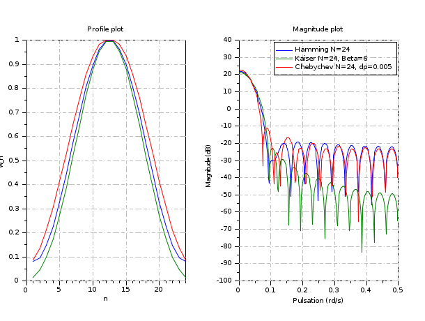
clf()
N=24;
whm=window('hm',N);//Hamming window
wkr=window('kr',N,6);//Hamming Kaiser window
wch=window('ch',N,[0.005,-1]);//Chebychev window
//plot the window profile
subplot(121);plot(1:N,[whm;wkr;wch]')
set(gca(),'grid',[1 1]*color('gray'))
xlabel("n")
ylabel("w_n")
title(gettext("Profile plot"))
//plot the magnitude of the frequency responses
n=256;
[Whm,fr]=frmag(whm,n);
[Wkr,fr]=frmag(wkr,n);
[Wch,fr]=frmag(wch,n);
subplot(122);plot(fr,20*log10([Whm;Wkr;Wch]'))
set(gca(),'grid',[1 1]*color('gray'))
xlabel(gettext("Pulsation (rd/s)"))
ylabel(gettext("Magnitude (dB)"))
legend(["Hamming N=24";"Kaiser N=24, Beta=6";"Chebychev N=24, dp=0.005"]);
title(gettext("Magnitude plot"))
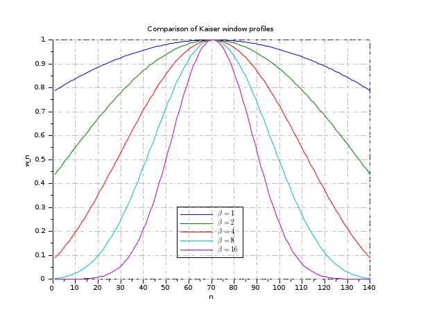
clf()
N=140;
w1=window('kr',N,1);
w2=window('kr',N,2);
w4=window('kr',N,4);
w8=window('kr',N,8);
w16=window('kr',N,16);

//plot the window profile
plot(1:N,[w1;w2;w4;w8;w16]')
set(gca(),'grid',[1 1]*color('gray'))
legend("$\beta="+string([1;2;4;8;16])+'$',[55,0.3])
xlabel("n")
ylabel("w_n")
title(gettext("Comparison of Kaiser window profiles"))
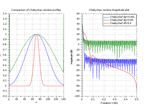
clf()
N=140;
w1=window('ch',N,[0.001,-1]);
w2=window('ch',N,[0.05,-1]);
w3=window('ch',N,[-1,0.4]);

//plot the window profile
subplot(121);plot(1:N,[w1;w2;w3]')
set(gca(),'grid',[1 1]*color('gray'))
//legend("$\beta="+string([1;2;4;8;16])+'$',[55,0.3])
xlabel("n")
ylabel("w_n")
title(gettext("Comparison of Chebychev window profiles"))
//plot the magnitude of the frequency responses
n=256;
[W1,fr]=frmag(w1,n);
[W2,fr]=frmag(w2,n);
[W3,fr]=frmag(w3,n);
subplot(122);plot(fr,20*log10([W1;W2;W3]'))
set(gca(),'grid',[1 1]*color('gray'))
xlabel(gettext("Pulsation (rd/s)"))
ylabel(gettext("Magnitude (dB)"))
legend(["Chebychef dp=0.001";"Chebychef dp=0.05";"Chebychef df=0.4"]);
title(gettext("Chebychev window Magnitude plot"))
See Also
Bibliography
IEEE. Programs for Digital Signal Processing. IEEE Press. New York: John Wiley and Sons, 1979. Program 5.2.
| Report an issue | ||
| << wigner | filters | zpbutt >> |