ode

Arguments

y0: a real vector or matrix: initial state, at t0.
t0: a real scalar, the initial time.
t: a real vector, the times at which the solution is computed.
f: an external function (Scilab function, list or string), computes the value of f(t, y). It is the right hand side of the differential equation. See f description section for more details.
type: a string, the solver to use. The available solvers are "adams", "stiff", "rk", "rkf", "fix", "discrete" and "root".
rtol: relative tolerance on the final solution y (decimal numbers). If each is a single value, it applies to each component of y. Otherwise, it must be a vector of same size as size(y), and is applied element-wise to y.
atol: absolute tolerance on the final solution y (decimal numbers). If each is a single value, it applies to each component of y. Otherwise, it must be a vector of same size as size(y), and is applied element-wise to y.
jac: an external function (a Scilab fuction, list or string), computes the Jacobian of the function f(t, y). See jacobian description section for more details.
ng: an integer, number of components of g function
g: an external function (a Scilab fuction, list or string) with the syntax g(t, y), returns a vector of size ng. Each component defines a surface. Used ONLY with "root" solver. See ode_root help page.
y: a real vector or matrix. The solution.
rd: a vector available ONLY with "root" solver. See ode_root help page.
w, iw: real vectors. (INPUT/OUTPUT). See ode() optional output.

Description

ode solves explicit Ordinary Different Equations defined by:

$\begin{eqnarray} \begin{array}{l} \dfrac{dy}{dt} = f(t,y)\\ y(t_0)=y_0 \end{array} \end{eqnarray}$

It is an interface to various solvers, in particular to ODEPACK.

In this help, we only describe the use of ode for standard explicit ODE systems.

The simplest call of ode is: y = ode(y0,t0,t,f) where

y0 is the vector of initial conditions,
t0 is the initial time,
t is the vector of times at which the solution y is computed
f defines the right hand side of the first order differential equation. This argument is a function with a specific header. See f description section for more details.
and y is matrix of solution vectors y=[y(t(1)),y(t(2)),...].

The tolerances rtol and atol are thresholds for relative and absolute estimated errors. The estimated error on y(i) is: rtol(i)*abs(y(i))+atol(i) and integration is carried out as far as this error is small for all components of the state. If rtol and/or atol is a constant rtol(i) and/or atol(i) are set to this constant value. Default values for rtol and atol are respectively rtol=1.d-5 and atol=1.d-7 for most solvers and rtol=1.d-3 and atol=1.d-4 for "rfk" and "fix".

For stiff problems, it is better to give the Jacobian of the RHS function as the optional argument jac.

Optional arguments w and iw are vectors for storing information returned by the integration routine (see ode_optional_output for details). When these vectors are provided in RHS of ode the integration re-starts with the same parameters as in its previous stop.

More options can be given to ODEPACK solvers by using %ODEOPTIONS variable. See odeoptions help for more details.

The solvers

The type of problem solved and the method used depend on the value of the first optional argument type which can be one of the following strings:

<not given>:: lsoda solver of package ODEPACK is called by default. It automatically selects between nonstiff predictor-corrector Adams method and stiff Backward Differentiation Formula (BDF) method. It uses nonstiff method initially and dynamically monitors data in order to decide which method to use.
"adams":: This is for nonstiff problems. lsode solver of package ODEPACK is called and it uses the Adams method.
"stiff":: This is for stiff problems. lsode solver of package ODEPACK is called and it uses the BDF method.
"rk":: Adaptive Runge-Kutta of order 4 (RK4) method.
"rkf":: The Shampine and Watts program based on Fehlberg's Runge-Kutta pair of order 4 and 5 (RKF45) method is used. This is for non-stiff and mildly stiff problems when derivative evaluations are inexpensive. This method should generally not be used when the user is demanding high accuracy.
"fix":: Same solver as "rkf", but the user interface is very simple, i.e. only rtol and atol parameters can be passed to the solver. This is the simplest method to try.
"root":: ODE solver with rootfinding capabilities. The lsodar solver of package ODEPACK is used. It is a variant of the lsoda solver where it finds the roots of a given vector function. See help on ode_root for more details.
"discrete":: Discrete time simulation. See help on ode_discrete for more details.

f function

The input argument f defines the right hand side of the first order differential equation. It is an external i.e. a function with specifed syntax, or the name a Fortran subroutine or a C function (character string) with specified syntax or a list.

a Scilab function

In this case, the syntax must be

ydot = f(t, y)

where

t is a real scalar (the time)
y is a real vector (the state)
ydot is a real vector (the first order derivative dy/dt).

a list

This form of external is used to pass parameters to the function. It must be as follows:

list(simuf, u1, u2, ..., un)

where the syntax of the function simuf is now

ydot = simuf(t, y, u1, u2, ..., un)

and u1, u2,..., un are extra arguments which are automatically passed to the function simuf.

a character string

It must refer to the name of a Fortran subroutine or a C compiled function. For example, if we call ode(y0, t0, t, "fex"), then the subroutine fex is called.

The Fortran calling sequence must be

subroutine fex(n, t, y, ydot)
double precision t, y(*), ydot(*)
integer n

The C syntax must be

void fex(int *n, double *t, double *y, double *ydot)

where

n is an integer
t is the current time value
y the state array
ydot the array of state derivatives (dy/dt)

This external can be build in a OS independent way using ilib_for_link and dynamically linked to Scilab by the link function.

The function f can return a p-by-q matrix instead of a vector. With this matrix notation, we solve the n=p+q ODE's system dY/dt=F(t,Y) where Y is a p x q matrix. Then initial conditions, Y0, must also be a p x q matrix and the result of ode is the p-by-q(T+1) matrix [Y(t_0),Y(t_1),...,Y(t_T)].

Jacobian function

For stiff problems, it is better to give the Jacobian of the RHS function as the optional argument jac.

The Jacobian is an external i.e. a function with specified syntax, or the name of a Fortran subroutine or a C function (character string) with specified calling sequence or a list.

a Scilab function

The syntax must be

J = jac(t, y)

where

t is a real scalar (time)
y is a real vector (the state)

The result matrix J must evaluate to df/dx i.e. J(k,i) = dfk/dxi where fk is the k-th component of f.

a list

This form of external is used to pass parameters to the function. It must be as follows:

list(jac, u1, u2, ..., un)

where the syntax of the function jac is now

ydot = jac(t, y, u1, u2, ..., un)

and u1, u2,..., un are extra arguments which are automatically passed to the function jac.

a character string

It must refer to the name of a Fortran subroutine or a C compiled function.

The Fortran calling sequence must be

subroutine jac(n, t, y, ml, mu, J, nrpd)
integer n, ml, mu, nrpd
double precision t, y(*), J(*)

The C syntax must be

void jac(int *n, double *t, double *y, int *ml, int *mu, double *J, int *nrpd)

In most cases you have not to refer ml, mu and nrpd.

Examples

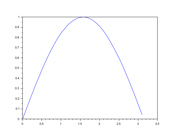
In the following example, we solve the Ordinary Differential Equation dy/dt=y^2-y*sin(t)+cos(t) with the initial condition y(0)=0. We use the default solver.

function ydot=f(t, y)
    ydot=y^2-y*sin(t)+cos(t)
endfunction
y0=0;
t0=0;
t=0:0.1:%pi;
y = ode(y0,t0,t,f);
plot(t,y)

In the following example, we solve the equation dy/dt=A*y. The exact solution is y(t)=expm(A*t)*y(0), where expm is the matrix exponential. The unknown is the 2-by-1 matrix y(t).

function ydot=f(t, y)
    ydot=A*y
endfunction
function J=Jacobian(t, y)
    J=A
endfunction
A=[10,0;0,-1];
y0=[0;1];
t0=0;
t=1;
ode("stiff",y0,t0,t,f,Jacobian)
// Compare with exact solution:
expm(A*t)*y0

In the following example, we solve the ODE dx/dt = A x(t) + B u(t) with u(t)=sin(omega*t). Notice the extra arguments of f: A, u, B, omega are passed to function f in a list.

function xdot=linear(t, x, A, u, B, omega)
    xdot=A*x+B*u(t,omega)
endfunction
function ut=u(t, omega)
    ut=sin(omega*t)
endfunction
A=[1 1;0 2];
B=[1;1];
omega=5;
y0=[1;0];
t0=0;
t=[0.1,0.2,0.5,1];
ode(y0,t0,t,list(linear,A,u,B,omega))

In the following example, we solve the Riccati differential equation dX/dt=A'*X + X*A - X'*B*X + C where initial condition X(0) is the 2-by-2 identity matrix.

function Xdot=ric(t, X, A, B, C)
    Xdot=A'*X+X*A-X'*B*X+C
endfunction
A=[1,1;0,2];
B=[1,0;0,1];
C=[1,0;0,1];
y0=eye(A);
t0=0;
t=0:0.1:%pi;
X = ode(y0,t0,t,list(ric,A,B,C))

In the following example, we solve the differential equation dY/dt=A*Y where the unknown Y(t) is a 2-by-2 matrix. The exact solution is Y(t)=expm(A*t), where expm is the matrix exponential.

function ydot=f(t, y, A)
    ydot=A*y;
endfunction
A=[1,1;0,2];
y0=eye(A);
t0=0;
t=1;
ode(y0,t0,t,list(f,A))
// Compare with the exact solution:
expm(A*t)
ode("adams",y0,t0,t,f)

With a compiler

The following example requires a C compiler.

// ---------- Simple one dimension ODE (C coded external)
ccode=['#include <math.h>'
       'void myode(int *n,double *t,double *y,double *ydot)'
       '{'
       '  ydot[0]=y[0]*y[0]-y[0]*sin(*t)+cos(*t);'
       '}']
mputl(ccode,TMPDIR+'/myode.c') //create the C file
// Compile
cd TMPDIR
ilib_for_link('myode','myode.c',[],'c',[],'loader.sce');
exec('loader.sce') //incremental linking
y0=0;
t0=0;
t=0:0.1:%pi;
y = ode(y0,t0,t,'myode');

Bibliography

Alan C. Hindmarsh, "lsode and lsodi, two new initial value ordinary differential equation solvers", ACM-Signum newsletter, vol. 15, no. 4 (1980), pp. 10-11.

Used Functions

The associated routines can be found in SCI/modules/differential_equations/src/fortran directory: lsode.f lsoda.f lsodar.f

Report an issue
<< numderivative	Differential Equations	ode_discrete >>

Syntax

Arguments

Description

The solvers

f function

Jacobian function

Examples

With a compiler

See also

Bibliography

Used Functions