polarplot
Plot polar coordinates
Syntax
polarplot(theta,rho,[style,strf,leg,rect])
polarplot(theta,rho,<opt_args>)
h = polarplot(...)
Arguments
- rho
a vector, the radius values
- theta
a vector with same size than rho, the angle values.
- <opt_args>
a sequence of statements
key1=value1, key2=value2, ... where keys may bestyle,leg,rect,strforframeflag- style
is a real row vector of size nc. The style to use for curve
iis defined bystyle(i). The default style is1:nc(1 for the first curve, 2 for the second, etc.).- -
if
style(i)is negative, the curve is plotted using the mark with idabs(style(i))+1. See polyline properties to see the mark ids.- -
if
style(i)is strictly positive, a plain line with color idstyle(i)or a dashed line with dash idstyle(i)is used. See polyline properties to see the line style ids.- -
When only one curve is drawn,
stylecan be the row vector of size 2[sty,pos]wherestyis used to specify the style andposis an integer ranging from 1 to 6 which specifies a position to use for the caption. This can be useful when a user wants to draw multiple curves on a plot by calling the functionplot2dseveral times and wants to give a caption for each curve.
- strf
is a string of length 3
"xy0".- default
The default is
"030".- x
controls the display of captions,
- x=0
no captions.
- x=1
captions are displayed. They are given by the optional argument
leg.
- y
controls the computation of the frame. same as frameflag
- y=0
the current boundaries (set by a previous call to another high level plotting function) are used. Useful when superposing multiple plots.
- y=1
the optional argument
rectis used to specify the boundaries of the plot.- y=2
the boundaries of the plot are computed using min and max values of
xandy.- y=3
like
y=1but produces isoview scaling.- y=4
like
y=2but produces isoview scaling.- y=5
like
y=1butplot2dcan change the boundaries of the plot and the ticks of the axes to produce pretty graduations. When the zoom button is activated, this mode is used.- y=6
like
y=2butplot2dcan change the boundaries of the plot and the ticks of the axes to produce pretty graduations. When the zoom button is activated, this mode is used.- y=7
like
y=5but the scale of the new plot is merged with the current scale.- y=8
like
y=6but the scale of the new plot is merged with the current scale.
- leg
a string. It is used when the first character x of argument
strfis 1.leghas the form"leg1@leg2@...."whereleg1,leg2, etc. are respectively the captions of the first curve, of the second curve, etc. The default is"".- rect
This argument is used when the second character y of argument
strfis 1, 3 or 5. It is a row vector of size 4 and gives the dimension of the frame:rect=[xmin,ymin,xmax,ymax].- h
This optional output contains a handle to a Compound entity which is described below.
Description
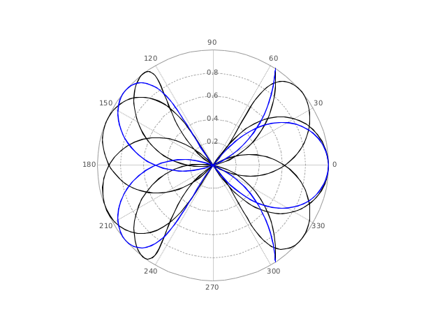
polarplot creates a polar coordinate plot of the angle theta versus the radius rho. theta is the angle from the x-axis to the radius vector specified in radians; rho is the length of the radius vector specified in dataspace units. Note that negative rho values cause the corresponding curve points to be reflected across the origin.
The optional output hcontains a handle to a Compound entity whose children are:
h.children(1): Compound whose children are the labels of angle values (Text entities)h.children(2): Compound whose children are the lines of radial frame for each angle value (Segs entities)h.children(3): Compound whose children are the labels of radius values (Text entities)h.children(4): Compound whose children are the circles of constant radius for each radius value (Arc entities)h.children(5): Polyline entity, the main curve.
h to modify properties
of a specific or all Text, Segs or Arc entites after they are created. For a list of
properties, see Polyline_properties,
segs_properties or
arc_properties.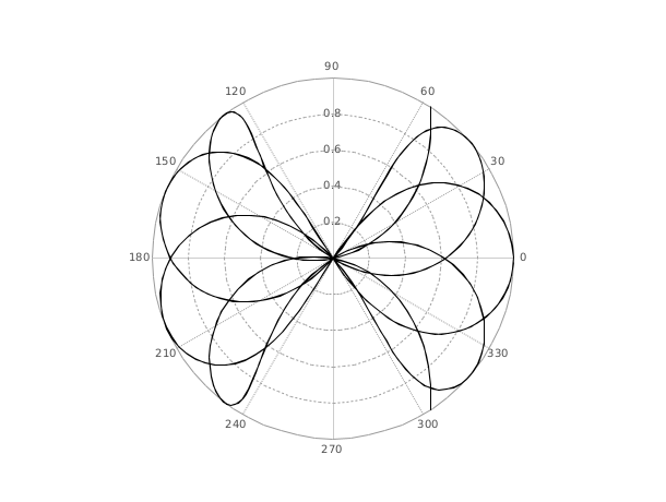
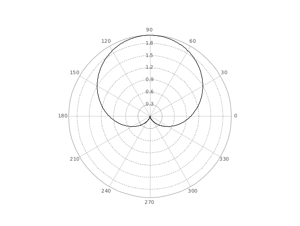
Example 4
clf
theta = [0:0.02:2*%pi]';
rho = 1+0.2*cos(theta.^2);
polarplot(theta,rho,style=5)
gca().data_bounds = [-1.2,-1.2;1.2,01.2];
History
| Версия | Описание |
| 2025.0.0 | Function returns the created handle(s). |
| Report an issue | ||
| << plotimplicit | 2d_plot | scatter >> |